The ABCs of Quantum Computing
Part A
This text is visible if you are not logged in to TIM. You can watch the videos, but you cannot do the exercises. Log in to TIM here:
You're looking at the first part of the ABCs of Quantum Computing. This part A focuses on the core concepts needed to understand quantum information and quantum computing. Quantum physics will be introduced as we go along. The actual mathematical theory of quantum physics will only be introduced in later parts, so you won't need much maths knowledge in this part.
Instead, many new concepts will be introduced. Think carefully about the content of those concepts, as well as the connections between them.
As a whole, the course consists of this one interactive document. Information is provided in both video and text formats. Near the start of the course there are more videos and text, and the number of interactive tasks increases towards the end. The course is largely based on learning by doing and requires you to take an active approach to your studies. Concentrate on the exercises and don't get discouraged if a task requires more than one attempt. In the final part you get to program a quantum computer simulator!
The videos in the document can be distinguished from the other images by the symbol at the bottom right . You can adjust the speed of the videos and turn on subtitles if you wish. You can find the tags at the bottom of the video and below the screen when you start the video.
About the document sections and their colouring:
- Some words are more important than others. The keywords are this kind of bold and dark blue. You can find the glossary in the menu bar at the top of the document.
- Try it yourself boxes let you do something yourself. Don't rush through these items, but take your time to think about what the thing in the box is about.
- The text is interspersed with mild questions as learning aids. You can answer a question only once, so guessing is not advisable. Go back to the text and videos if you don't know the answer. The questions are there to help you learn -- you will not fail the course if you answer incorrectly.
- You gain points by chewing tart and tasty exercises. You can do the exercises as many times as you need to. Some exercises require you to answer the question correctly three times in a row. You must complete all exercises to finish the course.
- The rocky path of learning is padded with moss green instructions and explanations. You may skip these parts if you feel you don't need the help. Occasionally you will be presented with additional information. This too is highlighted in green.
The right margin is reserved for your own notes.
You can write notes for yourself (Just me) or observations visible to others (Everyone). Click the text first. If the menu is on the right (default), click the pencil icon to open the menu and select ‘Comment/Note’ from there. If the menu is on the left, the letter ‘C’ will appear for commenting.
Quantum Owl's help
There are orange bars on the right-hand side of the page. The orange bar indicates a block that you have not yet read. Click on the bar to mark the block as read. If the teacher makes corrections and the block changes after you have read it, the bar will turn yellow. You can hide such an instruction by clicking on the owl. The tips and additional information boxes are closed and can be opened by clicking on the owl.
Below you will find a list of specific instructions. If you are already in a hurry to start the course, you can skip the following instructions and return to them only if you need to.
To complete the course, please review all the course material and in particular
test all Try it yourself boxes yourself
answer all questions (it is OK to answer incorrectly)
complete all of the exercises
at the very end, reflect on what you have learned and summarise the main points in a few sentences
Click Save after your activity whenever there is one in the box. This way your work will be recorded. Saving will also cause your answer to be checked. If your answer is wrong, then for the exercises, keep trying.
You can only answer a question once, so it's not a good idea to go off on a wild guess. If in doubt, go back to the text and videos or the 'try it yourself' box that accompanies the question. Of course, it's OK to get it wrong, but then you know you need a refresher. The purpose of the questions is to give you a chance to test that you've understood the point.
You can do the exercises as many times as you need to. The exercises will give you practice on the topics covered in the course. Typically, the insight sought in an assignment requires experimentation. When a gate assignment comes up, fearlessly try all the gates and inputs it allows. As a general rule, it is recommended to complete the exercises as they come up. You can also leave a difficult exercise for later. To pass the course, all exercises must be completed.
You can check your performance at the end of the document, where you will find a list of unanswered questions and unfinished exercises.
There are orange bars on the right-hand side of the page. The orange bar indicates a block that you have not yet read. Click on the orange bar to mark it as read. Click on ![]() to mark the document blocks up to the previous title level as read. If you don't like the bars, you can disable them completely by clicking on the wheel -> Mark all as read. However, the bars are the preferred way to keep track of your progress, so you should at least try using them.
to mark the document blocks up to the previous title level as read. If you don't like the bars, you can disable them completely by clicking on the wheel -> Mark all as read. However, the bars are the preferred way to keep track of your progress, so you should at least try using them.
If you need help with the course assignments or you need clarification on something, the right place to ask questions is the course discussion board. You can access the discussion board from the Discussion section in the top bar.
For many of the tasks, you will already find a hint under the task by clicking on the green owl. If you get stuck, ask for advice on the discussion board. It is worth checking the previous discussion first, as someone else may have already asked the same question.
Referring to a specific task is handy, for example, when you want to ask a question about it on the discussion forum.
In the top right-hand corner of the question, task and other sections, there is a # symbol. This is a link to that section. When you hover your mouse over the symbol, your browser will display the address of the link at the bottom of the screen or near the address bar. The section name is the one after the # symbol in the address. You can also click on the link. You will then see the name of the section in the address bar.
- Before you start watching the video, read the accompanying text next to or below the video (depending on the device you are using).
- Speed allows you to adjust the speed of the video.
- Adv allows you to see the forward and backward jump controls.
- Subtitles can be changed by clicking the three vertical dots (Chrome) or on the CC icon (Firefox).
- Hide file allows you to hide the video view after watching it.
The ABCs of Quantum Computing uses TIM as its platform. TIM (The Interactive Material) is a versatile learning platform that allows the creation of interactive learning materials. TIM is open source software maintained by the Faculty of Information Technology at the University of Jyväskylä. More about TIM can be found here. The essential thing for this course is that this TIM document contains different interactive tasks. In addition, you can modify the view of the document to some extent to your liking. The image in the upper left corner of the book shows the table of contents.
You can email the course organiser at kvanttiaakkoset@jyu.fi. There is also a feedback form at the end of the course.
Part A of the Quantum Computing Essentials has been created at the University of Jyväskylä, Faculty of IT. The TIM implementation of the course has been designed by Teiko Heinosaari, Juha Reinikainen and Vesa Lappalainen. Juha, Vesa and the TIM team have created the necessary building blocks for TIM. The course material has been designed and written by Teiko. The videos have been shot by Teiko together with Jari Niemi and Joni Palmiranta. Jari and Joni have edited the videos. Illustrations are the work of Aino Sutinen.
A.1 What is quantum physics?
We start the course with a brief introduction to quantum physics.
A.1.1 The beginning of quantum physics
Physics is a discipline that seeks to understand the universe and its phenomena at a fundamental level and to develop theories to describe and predict them. Physics is roughly divided into classical physics and modern physics. Classical physics includes mechanics, thermodynamics and electromagnetism. Mechanics studies the motion of bodies and the forces that cause motion. Thermodynamics deals with heat and energy changes. Electromagnetism studies electric and magnetic fields and their effects on charged bodies.
The pillars of modern physics are quantum mechanics and theory of relativity, which emerged in the early decades of the 20th century. Quantum mechanics and relativity are still being studied and developed. They have also given rise to new subfields of physics, such as particle physics and nuclear physics.
Physics research is typically divided into experimental and theoretical research. However, these are closely related and go hand in hand, sometimes focusing on the same research problems and sometimes intertwining. The field of physics is expanding in new directions, especially when observations are made that cannot be adequately explained by old theories. On the other hand, new theories lead to the search for new phenomena in a new way or from a new perspective. In physics research, experimental and theoretical approaches are both highly developed and equally important. Both played a role in the emergence of quantum physics. Nowadays, with the development of computers, computational physics can be further distinguished as a third approach and has become an important part of quantum physics research in addition to experimental and theoretical research.
Quantum mechanics was initially a theory explaining the behaviour of small objects, especially atoms. Later it was realised that in some situations the physics of large objects also requires the use of quantum mechanics principles. For example, some properties of black holes cannot be explained without quantum mechanics. Quantum mechanics therefore no longer means only the physics of small objects. In certain circumstances or situations, physics is different from classical physics, whether it is a large or small object.
Quantum Owl's help
The first question is below. You can only answer the questions once. If you don't know the answer, you should watch the video again. Getting it wrong is not that serious, though.
A.1.2 System, state and measurement
A physical system is an entitity, or a portion of the universe, whose function is sought to be understood by physics. A physical system is rarely separate from the rest of the world, but the physicist, in her mind, divides the world into the system under consideration and its environment. This division depends entirely on the particular issues of interest. A system interacts with its environment when its behaviour is changed in some way by the environment.

The starting point in physics is that the system under study is observed. The aim is to find regularities in the observations, and so the theory of physics can help explain and predict the observations. To structure observations, it is useful to introduce the concepts of state and measurement. These concepts are particularly important in quantum physics, although they also belong to other physics. These two concepts will be the starting point for learning quantum physics in this course.
In the video thermodynamics was mentioned. Are you unfamiliar with the word?
Thermodynamics is a branch of physics that deals with the changes in energy, heat and work between physical systems. Temperature, volume, pressure and their changes are often relevant in thermodynamical studies. For example, the internal combustion engine of a car, where the energy from burning fuel is converted into mechanical motion, is a typical application of thermodynamics.
The basic setup of a physical experiment is shown below. A physical system is prepared for measurement. The process is called preparation and it results in the system being in some state. We call this state the initial state. The initial state can be known or unknown, as long as a similar preparation can be used to repeat the experimental setup. In principle, physics describes situations that can be repeated. For each repetition, the measurement device gives a measurement result.
There may also be a third distinguishable element in the situation. After preparation, the system may interact with the environment either in a controlled way or spontaneously, partly uncontrolled. This interaction can be generally referred to as a process. In time, the process occurs before the measurement.
In the process, the state of the system changes. A process can be a well-planned event, where the system is allowed to interact with the environment in a controlled way, including controlling the duration and intensity of the interaction. A process can also be an uncontrolled event, where the system is allowed to interact with the environment in a way that it would like to avoid. Typically, this means that noise or alarm is introduced into the system state. A process can include both controlled and uncontrolled events.
Sometimes there may be an interest in the state of the system even after the measurement. In some measurements, the system is lost during the measurement. For example, in a measurement of the location of a photon position, the photon is destroyed by detection. In other measurements, the system may be preserved (see figure below). In this case, however, it must be remembered that the state of the system may change during the measurement. It may be possible to deduce the state after the measurement from the measurement result, but this is not always the case and the change may be random. In principle, one must be prepared for the fact that the measurement changes the state of the system. The information about the properties of the system obtained from the measurement is therefore related to the state of the system before the measurement and only partly to the state after the measurement.
This division between preparation, process and measurement is not unique to quantum physics, but describes a large variety of physical situations. In quantum physics, however, we need to be more precise than usual about what kind of situation we are talking about and what we mean by the terms. Our everyday experience does not help in the same way as, say, the mechanics of a throwing motion.
A.1.3 Special features of quantum physics
In classical physics, systems are either objects or waves. A small object is also called a particle. A physical system that obeys the laws of quantum physics behaves differently from what we are used to in classical physics. To emphasise this difference, we may refer to a quantum system when we mean a physical system that requires quantum physics to understand its behaviour. A quantum system, like an electron, is not a particle in the sense of classical physics. Nor is a quantum system a wave, although its behaviour has wave-like features in certain kinds of experiments. A quantum system is a completely new kind of system, which is worth trying to understand without overly relying on the concepts of classical physics.
A classical particle, i.e. a particle that obeys the laws of mechanics, has a specific position and velocity at any given moment, regardless of whether these quantities are measured or not. Of course, such a claim may be impossible to test experimentally, but the assumption of observer-independent properties is not incompatible with classical physics. Our everyday experience also supports the idea that the properties of ordinary objects are fixed at any given moment.

In contrast to the situation in classical physics, a quantum system always involves properties that do not have a fixed value, but it is only during a measurement that one of the possible values emerges. In the context of quantum theory, it would be problematic to assume that all properties of a quantum system are fixed before measurement. In quantum physics, the observer makes a choice to perform a particular measurement, and in doing so, they obtain some information about the state of the quantum system. No matter what the measurement is, an unknown state of the quantum system cannot be inferred from a single measurement outcome.
A.2 Randomness and probability
In quantum physics, predicting future events involves randomness. In a typical quantum physics experiment, we cannot predict the outcome with complete certainty, but only calculate the probabilities of possible alternatives. This is one of the key features of quantum theory and it is why we will discuss randomness and probability in this section.
A.2.1 Different levels of randomness
In our everyday experience, future events are often associated with a certain degree of randomness. We may talk about probabilities when our knowledge is incomplete or uncertain.

If we are absolutely certain about the course of an event, we do not need to talk about probabilities at all. For example, we can be certain that an apple will fall to the ground when I throw it in the air. In such situations, physics tells us the unambiguous outcome and the steps leading up to it, in this example the trajectory and flight time of the apple. In some other situations, predicting the outcome would be possible in principle, but too difficult in practice. Throwing a dice is a good example. In principle, it is possible to calculate the dice's flight and roll on the table using mechanics equations of motion, but rarely do we know all the factors affecting the landing, such as the dice's position and initial speed, with sufficient accuracy.
After watching the previous video, can you describe and give examples of the three levels of randomness?
Quantum Owl's help
Videos with refreshers or additional instructions are not behind the cover image, but can be found among the text as shown below. You can skip them if you are already familiar with the subject.
Then remember in particular what was said in the video about the randomness of quantum measurement and answer the following question.
A.2.2 Mathematical description of probability
Whatever is the cause of randomness, we describe randomness mathematically in terms of probabilities. A probability distribution relates to a situation or event in which there are several possible outcomes. The probability of each possible outcome is a number between zero and one, and a probability distribution lists these numbers. The extreme cases 0 and 1 relate to special cases:
- If the probability of an event is 1, it will definitely happen.
- If the probability of an event is 0, it will definitely not happen.
When the alternatives are chosen to be mutually exclusive but comprehensive in the sense that there are no other possibilities, the sum of the probabilities is 1. The probability distribution is thus a list of numbers, each of which is between zero and one, and together they sum to one.
As shown in the video, the probability of an event is the relative frequency with which that option occurs in a repetition test. A repetition test is when the same event is repeated several times under similar conditions. The higher the number of repetitions, the more accurately the probability describes the actual situation.
Probability distributions are conveniently represented by bar charts. The bar chart below is an example of a probability distribution where there are four possible options. The height of the bar indicates the probability of the option. You can move the cursor over the bar in the chart to see the exact number.
The probability distribution above is a list of [0.1, 0.2, 0.1, 0.6]. (Note that we use a dot for decimal numbers.) Below is another probability distribution. What is it in list form?
Sometimes probabilities are expressed as percentages. A percentage means one hundredth, so 1%=0.01. Thus, in a probability distribution, the sum of probabilities is 100%.
Have a look at the bar charts below. One of them is not a probability distribution. Can you identify it?
Quantum Owl's help
This is the first task. To complete the course, all exercises must be correctly completed. You can try as many times as you like. In this particular task, you must get three correct answers in a row.
A.2.3 Probabilistic information
Imagine I hand you a die. It is either a regular one, or weighted so that you cannot get the outcomes five or six. But you don't know which one it is.
In the next task, you have three dice. One of them is defective in that it does not give all the numbers on the roll. You don't know which of the three dice is the defective piece and the only way to find out is to roll each of them. You can't yet deduce the defective dice from one roll. You may be able to guess it, but it will be pure guesswork. Don't start guessing, but roll the dice as many times as you can to distinguish the defective one with certainty.
As the number of options increases, you typically need to perform more iterations to find out the probabilistic information. The next task is otherwise similar to the one above, but now there are eight dice. As in the previous task, roll the dice as many times as you can confidently distinguish the defective die.
Let's summarise our findings in this section. The number obtained from a dice roll is random. The numbers of a normal die and a defective die correspond to different probability distributions. This difference is not apparent on a single roll, but after several rolls we can distinguish between a normal and a defective dice. More generally, assumptions or claims based on probability can be tested by repeating an experiment or by observing a similarly repeated event several times.
A.2.4 Randomness in quantum measurement results
Measurement is a means of obtaining information about the state of a physical system. In classical physics, such as mechanics, the accuracy of measurements is not limited by the theory. However, the accuracy of measurement is affected by practical considerations and not all inaccuracies can be eliminated, so typically the measurement is repeated and the measurement results are reported as a distribution of results rather than as a single number. The number calculated from the theory can then be compared to the distribution. In a successful experiment, the distribution of the measurement results is narrow and the number given by the theory is in the middle of the distribution. The randomness of the measurement result is therefore related to the fact that the measurement accuracy is limited. For this reason, different measurement rounds can give slightly different results.
By quantum measurement we mean a measurement on a quantum system. As in physics in general, the purpose of a quantum measurement is to provide information about the state of the system under consideration. But in the case of a quantum measurement, the number given by a single measurement does not tell us much about the state of the system. Even from a theoretical point of view, the information provided by a measurement cannot be summarised in a single number.
Next, consider a quantum measurement with four possible outcomes. When measurements are performed many times, a probability distribution can be calculated from the measurement results. Since a single measurement outcome does not tell us much, it is better to think of the probability distribution of measurement outcome as the actual result of a quantum measurement, rather than a single measurement outcome. Surely, a single measurement will give us some measurement outcome, but only by repeating the measurement will we get out the information that a quantum measurement can give about the state as a whole.
Below is a probability distribution that could describe the result of a quantum measurement. In this case, there are four possible outcomes.
Collecting such a probability distribution of the outcome of a quantum measurement requires numerous measurement iterations. A bar chart can also represent a theoretically calculated prediction of the probabilities of the outcome of a quantum measurement.
Imagine a situation where you set out to make a particular quantum measurement and repeat the same experiment several times. After each measurement, the quantum system is prepared back to the initial state, so the experiment is repeated in the same way. After each measurement, the relative number of outcomes can be calculated to obtain the probability distribution of the intermediate state. This intermediate step approximates the final result when the measurement is repeated a sufficient number of times, for example 1,000 times. If the number of repetitions is small, the probability distribution of the intermediate step can deviate from the theoretical probability distribution by a large amount. The intermediate step probability distribution can therefore be thought of as a record of the measurement outcomes obtained so far. It cannot be used to predict future measurement results.
Next, let's look at how the relative quantities calculated from the repeated experiment gradually start to approach the probability distribution describing the actual measurement result.
Quantum Owl's help
Take your time to explore the 'Try it yourself' box. These exercises will not be graded, but they will set the scene for a future exercise.
In this experiment, we found that the probability distribution calculated from a few measurements can be quite different from the actual probability distribution representing the entire measurement result statistics. Let's practice interpreting the bar chart some more. In the exercise below there is a simulation of another quantum measurement together with four different probability distributions. You must make enough measurements to be able to choose the correct probability distribution with sufficient confidence.
Let's recap the lesson of this section. The measurement outcome from a quantum measurement is (except in special cases) random, so the measurement outcome may vary depending on the measurement round. Quantum theory predicts the probability distribution of the measurement outcomes, and this should be thought of as the actual end result of a quantum measurement. A single measurement gives only one measurement outcome, so several measurements must be made to determine the correct probability distribution.
A.2.5 Tarina Timin ennustuksista
Tässä välissä saat vetää hiukan henkeä ja lukea tarinan. Samalla voit miettiä vastikään läpikäytyjä asioita.
Ystäväsi Tim sanoo, että Köhniönjärven syvin kohta on ainakin 10 metriä. Sinun mielestäni näin ei voi olla. Kiista voidaan ratkaista mittaamalla pohjan syvyyttä. Ei ole olennaista onko joku jo ollut Köhniönjärvellä mittausretkellä vai ei, sillä järven syvyys on yksikäsitteinen fakta. Se pysyy samanlaisena kiistahetkestä mittaukseen asti, ainakin riittävällä tarkkuudella. Tarpeeksi kattavalla mittausretkellä pääsette luultavasti asiasta selvyyteen. Tuntuu varsin sopivalta sanoa, että joko sinä olet oikeassa tai Timi on oikeassa, ja näin on jo ennen mittausten alkamista. Tässä asissa on siten epätietoisuutta, mutta ei satunnaisuutta. Voihan olla niinkin, että Timi on käynyt mittausretkellä sinulta salassa. Ehkä hän siitä syystä haluasi lyödä asiasta vetoa.
Köhniönjärven syvyyden selvittyä päättätte mennä Killerille seuraamaan raveja. Timi tykkää ystävällishenkisestä kiistelystä, joten hän ehdottaa vetoa liittyen yhteen ravien lähtöön. Timi on perehtynyt päivän raveihin ja vakuuttunut, että suomenhevosori Ylistön Yrjänä on niin kovassa kunnossa, että voittaa oman lähtönsä. Et usko tähän, ja näin saadaan mukava väittely aikaiseksi. Tämä asia on siinä mielessä erilainen kuin Köhniönjärven syvyys, että Yrjänän voitto selviää vasta keskipäivällä orin päästessä kisaamaan.
Timillä saattaa olla tarkkanäköisiä havaintoja hevosista ja tilastoja aikaisemmista raveista. Perustelujen ollessa kattavia ei välttämättä kuulosta täysin väärältä kun Timi julistaa, että hän tiesi asian. Mutta ei kai hän sitä ihan täydellä varmuudella voinut tietää?
Jatkatte matkaa kirjastolle pelaamaan lautapelejä. Eräässä tiukassa lopputilanteessa Timi voittaa pelin sillä edellytyksellä, että heittää kuutosen. Hän heittääkin halutun tuloksen ja julistaa, että tiesi saavansa kuutosen. Mutta onko väitteessä mitään järkeä? Eikös nopanheiton koko idea ole se, että lopputulos on kokonaan satunnainen? Periaatteellisella tasolla Timi on voinut tietää nopan lopputuloksen jo heittohetkellä, tai ainakin antaa siitä tarkan ennusteen. Näin siis siitäkin huolimatta, että Timi ei olisi varsinaisesti huijannut. Nopan liikerata nimittäin noudattaa mekaniikan lakeja, ja niissä ei ole tilaa sattumalle. Satunnaisuus johtuu puutteellisesta tiedosta, joka siis nopanheiton kohdalla liittyy nopan heittokorkeuteen, alkuvauhtiin ja muihin sellaisiin Timin kontrolloitavissa oleviin asioihin. Ehkä Timi on harjoitellut tietynlaista nopanheittoa, mistä senkin tietää.
Lautapelivoitostaan riemastuneena Timi haluaa jatkaa kisaamista. Penäät reilua vedonlyöntiä, jossa ei voi ennakolta tietää lopputulosta eikä siihen vaikuttaa. Jonkun merkillisen mutkan kautta Timi on saanut radioaktiivista materiaa haltuunsa. Hän laittaa kahteen purkkiin sellaisen kobolttiatomin, joka jossakin kohtaa hajoaa ja muuttuu nikkeliksi. Nyt Timi ehdottaa vetoa siitä, kumman atomi hajoaa ensin. Ydinfysiikan tiedoilla voimme laskea todennäköisyyden sille, että toinen atomi on hajonnut tietyn ajan kuluttua. Esimerkiksi 5 vuoden kuluttua ainakin toinen atomi on hajonnut 75% todennäköisyydellä. Vedonlyönnin kannalta olennainen asia on se, että nykytiedon valossa ei ole mahdollista ennustaa sitä, kumman ydin hajoaa ensin. Radioaktiivisen koboltin hajoaminen nikkeliksi on satunnaisuutta aidoimmillaan. Jos on välttämätöntä lyödä Timin kanssa vetoa, niin ainakaan tässä viimeisessä kisassa hän ei voi saada ennakkotiedosta apua eikä vaikuttaa atomin hajoamiseen.
A.3 Information
Information encompasses data that can be communicated through messages, signals, or symbols. The transmission of information to others is absolutely essential to almost all human activities. Information cannot exist on its own without a physical carrier. This is why quantum physics comes into play when dealing with information. In this section we will go through the basics of information.
A.3.1 Amount of information
Sending or storing a long message is more difficult than a short message, which is why it is important to understand the amount of information and to describe it in an appropriate way.
Let's review the main points made in the video. The basic unit of information is a bit. Mathematically, a bit can have two values, 0 or 1. It is often useful to think of the amount of information in terms of making a choice between several options and expressing your choice to others. One bit can be used to express a yes/no answer. Two bits can be used to express a choice between four options, as there are four sequences of two bits: 00, 01, 10 and 11. This is enough to indicate, for example, the direction with the four main cardinal points, e.g. 00 = north, 01 = east, 10 = south, 11 = west.

Each new bit multiplies the number of options by two. Hence, four bits allow you to choose between 16 different options.
Five bits allow you to choose between as many as 32 different options. This is enough to select, say, a particular letter in the alphabet, and so we could translate the text into a string of five-bit chunks. This is in fact what happens in telecommunications: information is translated into a string of bits, sent to the receiver and finally the string of bits is translated back into text or an image. In addition to the alphabet, written text uses a number of special characters, such as !, ? and @. Today, the 8-bit character encoding is commonly used, and each 8-bit string can be used to indicate a choice from 256 characters. There are different character encodings, so it is always important to know which one is in use.
What if there are 3, 5, or some other number that is not a multiple of 2? You can't express three options with a single bit, but two bits is too many in the sense that it is enough to express four options. It has been proven to be a correct way to measure the amount of information using the logarithm of 2. We don't need this in this course, but if you want to know more, you can read below.
Three bits are enough to express eight options, since  . Written using the exponent notation, this is
  , where the number of bits is in the exponent. More generally,
  bits are enough to express
  options.
What if we want to know the number of bits needed when the number of options is given? The inverse of the exponential function is the logarithm. In the case of information, we use the base 2 in the exponent (since the information is expressed as a number of bits), so the corresponding inverse is the 2-order logarithm function. This is defined such that, given a positive number  ,
, ") for
for  for
for  . For example,
 =4") , for
, for  . The value of this 2-tailed logarithm is defined for all positive integers. Use the calculator below to compute its values in different cases.
You can use the calculator to make sure that the number of bits needed is an integer when the options are a multiple of two (i.e. 2,4,8,16...). In other cases, the 2-base logarithm gives a decimal number.
A.3.2 Physical bit
When we receive new information, for example news about world events, it usually doesn't matter how we get that information. Information is the same information, whether it comes from TV news or a newspaper. Although information is abstract in this way, it cannot exist in isolation, without some physical entity. Information must have a carrier, i.e. some physical system from whose state we can read the information. In physics, reading information means measuring the system.

The simplest message carries one bit of information. Again, a bit must have a carrier, i.e. a physical system in whose variable state the bit is written. A bit is also a system that has two distinguishable states and thus the potential to carry one bit of information.
There are many different aspects to choosing a medium for information. One important consideration is the desire to communicate information reliably and effectively. Our habits also drive our choices. Newspapers may not be a very effective way to communicate, but many people still prefer to read the news in a paper newspaper. The persistence of information and susceptibility to interference are also important considerations. The video talked about the position and temperature of the cup in terms of communication. What kinds of disturbances affect these imaginary ways of communicating? The temperature of the cup changes over time to the temperature of the room and therefore the message does not stay there for long. On the other hand, the cup may fall off the table due to a relatively small nudge and then the message based on its position is lost. The temperature of the cup would not change much if it fell off. So both ways of communicating have their pros and cons.
A.3.3 Information processing
In both communication and computation, information is processed, i.e. it is modified and transformed. In both cases, a bit string is first selected, then the bit string is modified according to some rules, and finally the bit string is read. From a physics point of view, reading a bit string means that a measurement is performed on the system carrying the information. An earlier illustration of a physical experimental setup serves also as an illustration of information processing. As an extension to the earlier illustration, we can think of the preparation device as having selection knobs that select a particular bit string and then prepare the physical system accordingly for a particular initial state. In physics terms, the process transforms the initial state into another state. Information processing is thus the transformation of a state in some systematic way.
The process can consist of several sub-steps. In the next section, we will practice building different processes from smaller pieces.
In communication, the sender and receiver are different persons and the process can be modelled, for example, by the noise of a communication channel. In such a context, the process is called a channel. For example, light can be transmitted by an optical fibre, which is then a communication channel.
We will henceforth denote by the letter q the bit string that is selected and according to which the physical system carrying the information is prepared for a state. The system is then passed through the process of measurement. Thus, the bit string q is the input of information processing. We also use the notation q[0] for the first bit of the bit string from the left, q[1] for the next bit, etc. For example, if q=100101110, then q[0]=1 and q[1]=0. Note that, in typical computer science fashion, we start counting the locations of the bits starting from zero. Let's practice this notation in the following exercises.
A.3.4 Binary numbers
One important form of information processing is computation. Computation refers to the process of performing mathematical operations on numbers. In this case, the input bit string represents a number, or a number of numbers. Numbers can be represented as bit strings in several different ways. If the purpose is to perform a computation, it is most convenient to represent numbers in binary form, where each number 0,1,2,3,... corresponds to a unique bit string. For example, addition for binary numbers is easy and we will look at the device that performs the addition later. When a bit string represents a number in binary form, we can write 2 in the lower right hand corner for clarity. For example,  corresponds to the number 42. We refer to as a binary number if the number is represented in binary form. When numbers are normally represented in base-10 format by the digits 0,1,2,...,9, only the digits 0 and 1 appear in the binary number. The binary form is therefore known as the base-2 format. The notation system is similar to that in conventional base-10 notation, i.e. the position of the digit denotes the multiples of the base number. Zero and one are the same in both formats, i.e.


All multiples of two in binary are simple, in the same way as multiples of ten (i.e. 100, 1,000, etc.) in the base-10 numeral system. So


In these multiples of two, the number of zeros tells you how many times two is multiplied. For example 16 is 2  2 2 2 so the binary representation has four zeros.
Let's then look at the numbers that are not multiples of two. Just as a number  in base-10 system can be decomposed into
  , the binary form of a number is obtained by adding together the multiples of the base. For example,
  as
as  and
and  ,
,  and
and  .
.
The numbers  are in binary format :


Can you extend the list further?
Did you work out how to get from one of the two different ways of representing a number to the other? Test your understanding with the following question.
Changing a number between different bases is fun. In this course, however, we will not focus on practising this any further. In the future, you can always use the number converter below if you need to. You can already test its use at this point.
A.3.5 A story about the starry sky of Singapore
Information is made up of bits. How could quantum physics change this? As we progress through this course, it will become clear that when information is carried by a quantum physical system, the nature of the information and how it is processed changes. We talk about quantum information when information is carried by a quantum physical system. The quantum physical equivalent of a bit is a qubit. We will introduce the qubit in section A.5.1 and then consider its difference from the bit. To keep things interesting we will tell an illustrative story first.
Your friend Timi likes to travel. He only knows of two possible destinations: the North Pole and the South Pole. Timi's favourite pastime is stargazing and the polar regions are perfect for that. At the North Pole, he particularly admires the Big Dipper. You can't see it at all from the South Pole and finding it in the sky is a sign to Timi that you are now at the North Pole. At the South Pole, Timi goes to admire the Southern Cross, which cannot be seen from the North Pole. Not only is Timi fascinated by these two destinations, but they are not even aware that there is anywhere else to go.

Timi thinks this is impossible - you would have to be at the North Pole and the South Pole at the same time! Your argument simply does not fit with what Timi thinks they know about the position of the stars and the possible locations of the Earth.
The difference between your and Timi's worldviews aptly illustrates the difference between a quantum physical system and an everyday system as a carrier of information. In the world of information, a bit has exactly two states, 0 (north pole) and 1 (south pole). A quantum physical bit, or qubit, has all of its superpositions in addition to these states. These superposition states can be likened to the fact that there are many more locations on the Earth than just the two poles. Just as Singapore does not have a north pole and a south pole at the same time, a superposition state is not 0 and 1 at the same time. Superposition states are a new kind of state not encountered in the bit world. Superposition states do, in a sense, lie between the bit states 0 and 1. This 'being in between' manifests itself in the fact that the observations of the states through measurements are something in between the observations that we would get through similar measurements on states 0 and 1 separately. Again, in this sense, the case corresponds to the fact that there is some similarity between the observations made in Singapore (the Big Dipper and the Southern Cross in the sky) and those made at both the North Pole and the South Pole. There are, however, also some differences (the constellations are in different places in the sky).
The qubit's superposition state is not a fuzzy state at all, nor is your loitering in Singapore. Sometimes the superposition state is described as the coincidence of states 0 and 1. This is not a good analogy though, since the quantum system is only in one state at a time. Each superposition state is just as valid a state as 0 and 1.
A.4 Gate array computation
In this section we will learn about computation based on gate arrays, or circuits, which is one model for computing and more generally for information processing. The rest of the course will include more exercises than before. You will become most familiar with gate arrays and quantum gate arrays when you adequately test different things on simulators.
A.4.1 Circuit simulator
One way to model information processing is to think of it as a sequence of successive changes, where these changes individually are simple or at least easy to model. We call the single device that causes a change a gate. The name refers to the fact that physical bits pass through these devices. Each gate changes one or more bits in some way. The actual implementation of the gates depends on the physical system into which the bits are encoded. For us, the essential thing is the model for information processing provided by the gate arrays and we do not care about the physical implementation.
In the following experiments and tasks we will use the circuit simulator, also referred as gate simulator. In the simulator you can change the input. The input is a bit string on the left side of the simulator. On the right side is the measurement. The value of each bit is measured separately, and together they make up the output. Information is processed between the input and output. Information processing happens in stages, and we call these steps. At each step, you can set gates that change the values of the bits. Steps can also be left blank, and then nothing happens at them.
As we agreed earlier, q denotes the bit string that is the entire input, and for example q[0] denotes the first bit of the input. When talking about the circuit simulator, q[0] refers to both the bit in question and the bit value. This will not cause us any confusion.
The gate simulator looks like this:
You can change the input value for each bit from zero to one and back by clicking on the box. The exception are bits with light-coloured edges. You cannot change their value.
Sometimes you are advised to put the gates in a row. This means that they affect the same bit (or bits) at different steps.
The gates used vary from one task to another. You don't need to go into the simulator manual (the circled question mark on the right side of the simulator) at this point, as we will practice using the simulator step by step. By pressing Save button, the gates you have drag and drop will be stored. Saving is a sign that you have completed the "Try it yourself" -box. For the actual tasks, saving will trigger a task review and scoring.
Reflect on the description you heard in the video about gate computing and answer the following question.
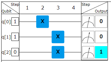
A.4.2 The X gate
A one-bit gate is the X gate. You will now be able to find out how it works independently.
Please
Try it yourself
In the simulator below you can drag the X gate to different locations and change the input. What does the X gate do to the bit? How can you describe its function in words?
Expand by moving mouse over the exercise or by clicking
The X gate is a very common gate and has several names depending on the context of use. Another common name for an X gate is NOT gate. Using the previous simulator, examine what two consecutive X gates do to an input and then answer the question below.
Does it feel easy or does the X gate cause difficulties? Let's take a watch the video for a summary of how the X gate works.
Try three more X gates in a row. Change the input and answer the question below.
Next, you will be presented with your first gate simulator exercise. The Save button will check your solution attempt. If it is wrong, you can try again. There is no limit to the number of attempts.
Quantum Owl's help
The general instruction for gate exercises is: experiment, experiment, experiment. By experimenting, you will learn how the gates work. The correct answer to the task will start to emerge through experimentation. But stop at the end to reflect on why the correct answer is what it is.
Please
Exercise
Use the X gates in a way that the input q=110 results in the output 101. Input and output are read from the 'in' and 'out' columns, starting from the top.
Expand by moving mouse over the exercise or by clicking
Let's do another similar exercise.
Please
Exercise
Use the X gates in a way that the input q=101010 results in an output of 100100.
Expand by moving mouse over the exercise or by clicking
You will find hints from the Quantum Owl under some of the exercises. You should not look at the hints right away, but try to do the exercise without it first.
In the exercise above, the first thing to do is to enter q=101010 as input. Then place the X gates so that the output is the desired one.
A.4.3 The swap gate
A gate can affect more than one bit at a time. In this case, the change to a single bit can also depend on the value of another bit. Two-bit gates are essential, especially in computing, because with single-bit gates alone, the input bits remain separate and can't do much useful work. Next, you'll explore the workings of one two-bit gate.
Please
Try it yourself
Drag a two-bit gate to the desired location and vary the values of the input. What does this gate do to the bits? How can you describe its function in words?
Expand by moving mouse over the exercise or by clicking
The gate above is called the swap gate. Swap means to exchange, so the name is very descriptive for that gate. The swap gate could also be modelled as a gate where the routes change places. Like so:
We will use the line connecting the two Xs to represent the swap gate, as it is easy to move and modify. Did you notice that you can stretch the gate after you have put it in place by moving one end further away? Try it and do the exercise below. Remember that the input is read from top to bottom in the simulator.
What does it mean by affects q[0] and q[2]? Does it mean connect these two? Because if i connect them, no answer is taken as correct. For example if i swap q[0] and q[2] the answer straight forward. But i am not sure whether the question means that. Could you please clarify?
—Then examine two consecutive swap gates that affect the same bits. Use the simulator above and put two swap gates in a row. Vary the inputs and see what the total effect of the gates is.
Place the swap-gates at different steps. For example, in steps 2 and 3. Place the gates so that the upper x in each is at bit q[0] and the lower x is at bit q[1]. 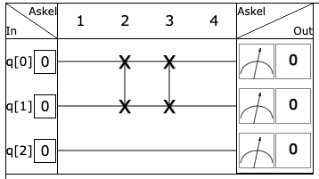 Now the gates are consecutive and affect the same bits. Investigate the interaction of the gates by trying through all possible inputs.
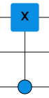
Let's continue with the exercises. In the following exercise, two different swap gates mean that they do not affect the exact same bits. There are three different swap gates for three bits and they look like this:
Please
Exercise
Use two different swap gates in a way that the input q=100 results in an output of 001 and input q=001 results in an output of 010.
Expand by moving mouse over the exercise or by clicking
Now that we've explored the two different gates, we can drag them both into the gate simulator. In the following exercise you will be able progress by experimenting with different combinations of gates to find the desired function.
Please
Exercise
Use the X gates and the swap gate so that input q=00 gives output 11, input q=11 gives output 00, and the other two inputs pass through unchanged.
Expand by moving mouse over the exercise or by clicking
The assignment includes a crucial hint about the number of ports: "..X gates and swap gate..". So it's enough to use one swap gate. Put it, for example, at step 2, and you can fit X gates on both sides. Then just try putting one, two or three X gates at different places. By varying the input, you can test how the combination works.
A.4.4 The CX gate
Another two-bit gate is called control-X or just CX. Also CNOT is one of the nicknames for this gate, remember that the X gate was also called the NOT gate.

The swap gate we tried earlier works symmetrically on both bits. The CX gate, on the other hand, is not symmetrical, as its symbol implies. Examine how the CX gate works yourself.
Please
Try it yourself
In the simulator below, make a CX gate by connecting the X gate to the control bit using a ball. Then examine the operation of the gate by varying the input. Why is the bit at the ball called the control bit?
Expand by moving mouse over the exercise or by clicking
Did you figure out how the CX gate operates? Let's go over once more what it's all about.
The CX gate consists of two parts, the control ball and the X gate. If the value of the bit in the control ball is 0, then the X gate has no effect on the other bit. If the control bit has a value of 1, then the X gate works like a normal X gate. So the control ball is like a switch that turns the X gate on or off.
Did you notice that in the CX gate, the control ball does not have to be on the bit closest to the X gate?
The swap gate we tried earlier works symmetrically on both bits. The CX gate, on the other hand, is not functionally symmetrical, as its symbol suggests. Next, examine the function of the CX gate.
Here also, the question says use x on q[2] and control on q[0] but then the result is fixed right? If i put the same in all the places also gives the same result. I am confused what is expected in this?. Could you please clarify?
—We may want to copy the value of one bit to several other bits. When the value of one bit is copied to two others, the desired function is:
Note that we ignore inputs other than 000 and 100, so the bits to be reproduced are in initial state 0. Initial state 0 corresponds to blank white paper fed into a standard copying machine.
Let's look at building a bit copying machine in the next exercise.
Please
Exercise
Use two CX gates and find a configuration such that the value of the first bit q[0] is copied to the next two bits when they are in initial state 0. When you have completed the circuit, press 'Save' and your solution will be checked.
Expand by moving mouse over the exercise or by clicking
As stated in the assignment, the idea is to use two CX gates. You can take your time to try out the different options and explore how they work. In copying, the first bit determines what happens to the others. Does it sound more natural to put an X gate or a control ball at that point? The bottom two bits have the same role, so they should be affected by the gates in the same way.
In the previous exercise, we saw that combining two-bit gates produces a result where three bits are connected together. Usually we get by with one- and two-bit gates, which can be placed in series to form entities that affect more than one bit. Sometimes gates acting on multiple bits come into play, and next we'll look at one of them.
A.4.5 The CCX gate
Did you notice that you can connect more than one control ball to the X gate? When two control balls are connected to an X gate, it is called a CCX gate. In this combination, the X gate and the control balls must be on the same step. The CCX gate is thus a three-bit gate. This gate also has several nicknames, and one of them is the Toffoli gate. Examine the operation of such a gate yourself.
Please
Try it yourself
In the simulator below, make a CCX gate by connecting two control bits to the X gate. Then examine the operation of the gate by varying the input.
Expand by moving mouse over the exercise or by clicking
Three different CCX gates can be made for three bits. These differ in which two bits are the control bits and which are affected by the X gate. Use the simulator above and find the right kind of CCX gate each time in the following exercise.
The CCX gate affects three bits. Of these, one becomes the X gate and the other two the controls. There are therefore three different CCX gates and they look like this: 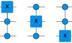
In the following exercise, you will have to experiment with different combinations of CCX gates and find the appropriate one.
Please
Exercise
Put two different CCX gates in series so that the input q=110 results in an output of 111 and the input q=111 results in an output of 011.
Expand by moving mouse over the exercise or by clicking
Two CCX gates in a row could look like this: 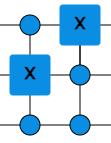 Try the assignment inputs for this combination of gates. If the output is not correct, then change the CCX gates.
A.4.6 Circuit
When multiple bits are used and many gates are connected in series, we call this entity a circuit. In circuit operation, we are interested in how different bit strings change as they pass through the circuit, i.e. what the output is for all possible inputs. Two different circuits, i.e. different combinations of gates, can lead to the same result. This means that they give the same output for all possible inputs. It is often the intention to try to achieve the desired function with the smallest possible number of gates. Sometimes other considerations favour the use of certain gates over others. For example, one gate may be easier to build than other gates. For example, it may be that two-bit gates can only be built between nearest neighbours due to the implementation. Other two-bit gates will then have to be assembled from these.
In gate array computation, the circuit corresponds to the overall process. Performing a particular information processing task may require a large number of gates, since the gates alone are simple in function. There may be many gates in a circuit and it is often not easy to deduce their interaction by looking at the circuit. In gate simulator tasks, it is worthwhile to experiment with the operation of a given circuit by varying the inputs, or to test different combinations of gates if you have to build a circuit.
Please
Try it yourself
Investigate the operation of the circuit below by varying the inputs. What does the circuit do? Changing the value of which bit affects the other bits?
Expand by moving mouse over the exercise or by clicking
The circuit above has four gates, but it can actually be operated with a smaller number of gates. Would one gate be enough, or do you need two?
Please
Exercise
Make a circuit with exactly the same function as the circuit above. This means that the outputs are the same as the circuit above for all inputs.
Expand by moving mouse over the exercise or by clicking
You can make a suitable circuit with just one gate. So you only need one step to make the circuit. You should be familiar with all the available gates, so go back and try to identify the circuit you are given. Did you notice that changing the value of bit q[1] has no effect on the other bits, nor does changing the other values have an effect on it? So you should first try a gate which does nothing to q[1]. You can connect bits q[0] and q[2] to each other using either a swap gate or a CX gate. Which of these does the given circuit resemble?
Let's do another similar exercise. Now the circuit is more complex. Keep your head cool and test how it works. The circuit is simple even though it consists of eight gates.
Please
Try it yourself
Investigate the operation of the circuit below by varying the inputs. What does the circuit do?
Expand by moving mouse over the exercise or by clicking
Please
Exercise
Make a circuit with exactly the same function as the circuit above.
Expand by moving mouse over the exercise or by clicking
As in the previous task, you can make a suitable circuit with just one gate. Test the given circuit enough to identify it. Which bits are such that changing them does not affect the others, and changing others does not affect them? One of the bits is such that changing it also affects another bit. The two bits must then be connected to each other with a suitable gate.
Even if the two circuits have exactly the same gates, they may not work in the same way. The final result is also affected by the order of the gates. Let's look at this next. Let's build two circuits with the same gates, but in a different order.
Please
Try it yourself
The top two bits are affected by swap and CX in sequence. In the two lower bits, put these gates in the opposite order. Then try different inputs with similar bit values going to these gate pairs, i.e. q[0]=q[2] and q[1]=q[3]. Does the different order of the gates have an effect on the output?
Expand by moving mouse over the exercise or by clicking
In the situation described in the question, two gates are placed in series, but in a different order. If q=1010 is chosen as the input, then both the upper and lower circuits receive the same input of 10. The output shows that the two two-bit circuits work differently. What other inputs give different results? Remember that we want to send the same input to the upper and lower circuits, so we are interested in inputs with q[0]=q[2] and q[1]=q[3]. 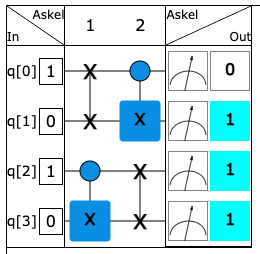
As we saw above, the order of the gates matters: the same gates placed in a different order may form different circuits.
As we already saw at the beginning of this section, two very different circuits may give exactly the same output for all inputs. The next task is to build a circuit that has the same functionality as a swap gate, but with only CX gates. So the same result can be achieved by using completely different gates. This task may require several attempts. First, however, you should refresh your memory on how the swap gate works in chapter A.4.3, so that you know the desired result.
Please
Exercise
Using multiple CX gates, create a circuit with the same function as a single swap gate. Try different configurations and find one where all possible inputs have the desired output.
Expand by moving mouse over the exercise or by clicking
The assignment recommends using multiple CX gates. You can position each CX gate in two ways: either the control ball is at the top or at the bottom. However, only the positioning of the gates is relevant for the desired function, since the swap gate works symmetrically. Thus, two CX gates can form a circuit where the control balls are on the same side or on different sides. Try these two options first. If neither circuit works as a swap gate, go to three CX gates. These either have all control balls on the same side or one is on a different side from the other two. A different CX gate can be first, middle or last. This makes four different circuits with three CX gates for the task.
A.4.7 Error correction
Imagine you and your friend Timi are sending messages. The messages are long strings of bits, encoded with things that are important to you in cipher. There has clearly been a glitch in the communication and you soon realise that there is interfering noise in the communication channel. The noise causes some bits to change in value between transmission and reception. For example, the bit string 1011101 changes to 1001101. This is where the value of the second bit has changed. A change in value is quite rare, but still very annoying, because the content of the message can then change completely. Can you think of a way that you and Timi can fight errors?
One possible way is to send each bit as a double or even a triple. You and Timi are already familiar with the ability of the CX gate to copy the value of a bit into multiple bits introduced in chapter A.4.4, so you can automate the multiplication. Sending a double may not be useful, because if one of the bit values changes, the correct value cannot be identified. Sending a triple, on the other hand, already has advantages. For example, the bit string 1011 is sent as 111000111111 . The change of one bit value in each of the three bit clusters due to noise is not a disadvantage because the receiver can then select the most frequent value in each of the three clusters. Since we assume that value changes are rare, a change of two bits in the same three clusters is very rare. Such a rare event would cause an error in the communication.
If necessary, we can switch to using multiplication by even more than three. In the following exercise, however, we will assume that you and Timi have found that multiplication by three is sufficient.
Here. The answer was taken as correct , but the is need to enter 3 times and the second time the same answer is taken as wrong and the whole exercise is set as not completed.
—The error-tolerant communication method between you and Timi can be automated. Copying a bit value into three is done by a copying circuit introduced in chapter A.4.4, and so is selecting the most frequently occurring bit value. The circuit below does just this latter operation: it selects the most common of the first three bit values in the input.
Please
Try it yourself
In this circuit, the first three bits are the input. The other bits are auxiliary bits and their value is fixed to zero. Change the input. This will change the values of all the bits in the output. One of the output bits is the one that indicates the most common value in the input. What is this output?
Expand by moving mouse over the exercise or by clicking
The input is the first three bits, i.e. bits q[0], q[1] and q[2]. The purpose of the circuit is to extract the most frequent input value. For example, if q[0]=0, q[1]=1 and q[2]=0, then 0 occurs twice and is the most frequent value. As you vary the input values, the output bits change. One of these outputs gives the most frequent value. Try sufficiently many different inputs to find the output that gives the most frequent value.
The previous circuit that selects the most common bit value is not simple. Timi tried to build the circuit, but remembered the connections wrong and did some parts differently. In the circuit below, you can't change the gates that Timi has already put there, but you can add gates to the empty steps. You need to complete the circuit in such a way that it works like the previous circuit, i.e. it can select the most common value of the first three bits. Note that the circuit cannot be externally identical because of the gates that Timi has connected. The values of the auxiliary bits do not matter.
Please
Exercise
Complete the circuit so that it gives the most common value of bits q[0], q[1] and q[2] to the same output bit as the previous circuit.
Expand by moving mouse over the exercise or by clicking
First of all, compare the given draft with the previous one. From this you can already draw conclusions about what kind of gates are missing in the given circuit. Will the empty steps be X, CX or CCX? When you consider the previous circuit, bits q[0], q[1] and q[2] are the actual inputs. Of the remaining five bits, one indicates the value of the most common bit occurring in the input and the other four are the auxiliary bits. In Timi's attempt, these auxiliary bits are in a different order than in the original circuit. So for the auxiliary bits, think about which auxiliary bit replaces which. Then make it so that the auxiliary bits with the same role have similar gates.
A.4.8 Addition
One of the most important functions of information processing is addition. Even complex calculations can be reduced to the addition of numbers, making a device performing addition a useful tool. So it's time to look at performing addition in circuit computations.
Adding up binary numbers is easy for both humans and computers. It is essential to know the results of the following simple addition operations. If necessary, rehearse the binary representation of numbers in chapter A.3.4 and, if you wish, you can change the numbers to a base-10 format to choose the correct answers in the table below.
Two larger binary numbers can be added with column addition. The addition then returns to the simple additions in the table above. The principle is the same as for the addition of numbers in base 10, but the method is easier because there are only two numbers.
First, let's recall how to do column addition in base 10. Let's add the numbers 219 and 1822. Let's write the numbers one below the other so that the 'ones' are on the same column, i.e. the numbers 9 and 2 are aligned vertically. The result of the calculation is written under the line.
  219
+1822
-----
The calculation proceeds from right to left. The numbers on the same column are added together. If the sum is 10 or more, we carry the 1 to the next column on the left.
   1
  219
+1822
-----
    1
We continue adding like this to the end.
 1 1
  219
+1822
-----
 2041
Column addition for binary numbers works in the same way.
Adding binary numbers is easy, and with the previous instructions you should be able to add binary numbers together with pen and paper. But we should let the machine do the work and look at a binary addition simulator.
Because of the memory row, a three-bit addition is needed to perform the colum addition. Did you already understand what a memory row is? Do the following exercise using the calculator above.
Since addition returns simple sums, it is sufficient to have a circuit that adds up the five simple sums of the previous table. By repeatedly using this circuit, we can then build a device that calculates the sum of even long binary numbers. The circuit must take two bit values A and B, and possibly a third bit value C from memory, since in the column calculation the previous sum may have left 1 in memory. Such a circuit is built below.
Please
Try it yourself
The circuit below implements a binary addition of two bits A and B, so that the value of the third bit C can be added from memory. Examine the operation of the circuit by varying the values of the first three bits and verify that the circuit works as desired. In the circuit, Cin is the value of the memory input and Cout is the value of the memory output. In the output, S is the last bit of the sum, that is, the bit that falls below the line in the column.
Expand by moving mouse over the exercise or by clicking
Let's add up the numbers 39 and 22. In binary, these are 100111 and 10110. Let's put them under each other first.
In the first step, the rightmost vertical line is calculated. Using the circuit above, the input is A=1 and B=0. In the first calculation, there can be nothing in memory yet, so Cin=0. Since 1+0 = 1, then S=1 and Cout=0.
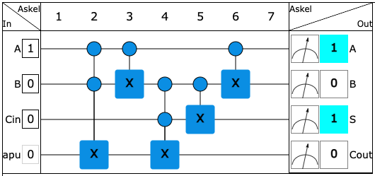
Let's put S below the line and Cout in memory.
In the next step, the circuit feed is A=1, B=1 and Cin=0. Since 1+1=10, then S=0 and Cout=1.
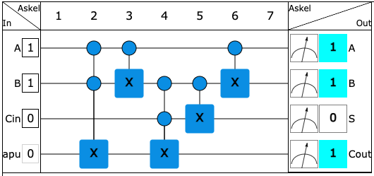
Again, let's put S below the line and Cout in memory.
In the next step, A=1, B=1 and Cin=1. Since 1+1+1=11, then S=1 and Cout=1.
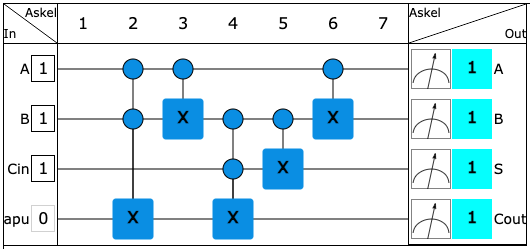
Let's put S under the line and Cout in memory.
This is how the calculation progresses. The circuit is used once for each column.
Addition usually ignores information in the sense that, for example, 4+5 = 9, but you can't tell from the result 9 whether 4+5 or, say, 3+6 were added together. The circuit described above does not lose information. This means that for every possible output you can uniquely infer the input. The reason for this is that we keep the values of A and B in the output. For a pure addition result, only the sum and Cout would be sufficient, as these are the only ones needed for the next step of addition in columns. However, you may want to use the numbers for some other calculation, so keeping them is useful.
Here also the second time the same answer is set as wrong and the whole exercise is set as incomplete
—Here the output is 0110 and the input will be 0100 as can be seen from the simulator above. But the question is marked as incorrect..and the exercise incomplete
—Binary addition of two bits can be done more easily if there is no third bit value in memory and no need to leave the input in memory unchanged, as above. Such a simpler circuit can execute the top four columns of the table. However, it cannot be used for addition in columns, since the addition of the fifth column  will not work. A binary sum of two bits is either 00, 01, 10, where for consistency we mark all zeros as visible. In the following exercise, S is such a sum marked with two bits. (For example, if A=1, B=0, then S=01 and hence S[0]=0 and S[1]=1.)
Please
Exercise
Build a circuit that performs the addition of two bits A and B such that A passes through as a variable, S[0] is the left bit of the sum and S[1] is the right bit of the sum.
Expand by moving mouse over the exercise or by clicking
The circuit we looked at earlier adds two bits together and even does the addition of the bit from memory correctly. The task asks you to make a circuit that does only part of this. It's worth trying different pieces of the earlier circuit and seeing which piece does the desired calculation.
The desired circuit should work as follows:
- A=0, B=0
 S[0]=0, S[1]=0
 - A=0, B=1 S[0]=0, S[1]=1
- A=1, B=0 S[0]=0, S[1]=1
- A=1, B=1 S[0]=1, S[1]=0
In all cases, the value of A must pass through unchanged.
A.5 Quantum gate array computation
In this section, we will look at the quantum physical version of gate array computation, i.e. quantum gate array computation.
A.5.1 Quantum bit or qubit
We have previously stated that information cannot exist without a physical system, but must have a physical carrier. The information can also be carried by a quantum system.
Just as with other physical systems, information is written into a quantum system by preparing it in a suitable way. Similarly, information is read by a suitable measurement. The simplest possible quantum system has only two perfectly distinguishable states. Such a system is called a quantum bit, or a qubit.
A qubit has an infinite number of states in total, and this distinguishes it essentially from a bit. A qubit is a bit-like information carrier in the sense that each state has exactly one orthogonal state, i.e. another state that can be completely distinguished from it. Thus, a single qubit can only transmit one bit of information. However, the information written in a qubit can be processed by quantum physical operations, and this makes even a single qubit a different information carrier from the physical manifestations of the bit that we saw earlier.
When two orthogonal states of a qubit are chosen, they can be thought of as bit states 0 and 1. In processing, these states can be transformed into superposition states, which are combinations of states 0 and 1. In these superposition states, the qubit does not have a fixed bit value, but the measurement randomly yields 0 or 1. It should be emphasised that the qubit is only in one state at any given time. The properties of that state may be such that the state resembles the 'zero' and 'one' states simultaneously, to a certain extent. In a superposition state, these two features may exist with different weights, and hence there are an infinite number of different superposition states.
All the gates we went through earlier work for qubits, but their operation for superposition states is not the same as for bit states 0 and 1. In chapter A.4.4 we inspected at a copying circuit which enables us to copy a single bit state to one or more other bits. However, the copying circuit does not copy superposition states into two identical superposition states. This is one of the main differences between a bit and a qubit in terms of information processing: you can copy the state of an unknown bit, but you cannot copy the state of an unknown qubit. Thus, the error correction introduced in chapter A.4.7 is also not as easy as with bits; for qubits, we need to invent novel methods.
In addition to superposition, quantum systems have another feature that distinguishes them from systems in classical physics. Several qubits can exist in a common quantum state that cannot be written as a combination of individual qubit states. In this case, the states of two or more qubits are entangled and their common state is called an entangled state.
A qubit can be implemented in many different quantum physical ways. For example, different implementations of a qubit can be made from interconnected superconducting electrodes. When we talk about a qubit, we are not referring to any particular physical implementation, but, as in the case of a bit, to any system that implements a qubit.
Next, we'll move on to using the quantum gate simulator. Capabilities of qubits will become apparent as we do the exercises. We won't get into the actual mathematical description until Part B.
A.5.2 Quantum Gate Simulator
Quantum gate computing is similar in principle to gate computing: changes are made to the information-carrying system in steps and finally a measurement is performed. Instead of bits, quantum gate computing processes qubits.
Let's review the main points of the video. The usual initial state for a qubit is some selected orthogonal states corresponding to bit states 0 and 1. We denote the values of the input as  and
and  as a reminder that we're doing quantum gate computation instead of regular gate computation. This notation originated with Paul Dirac, one of the founders of quantum mechanics, and has remained in use by quantum physicists. The usefulness of this notation is better illustrated in Part B of the Quantum Computing Essentials.
When the computation is started, the qubits are prepared into states corresponding to the input. At the end of the processing, a measurement is performed and the output is a bit string. The fact that the qubits are in superposition states prior to the measurement is reflected in the fact that the output of the measurement is random. The output of a quantum measurement is therefore best understood as a probability distribution, as was already discussed in chapter A.2.4.
All the gates we have previously explored function as such in quantum gate computation. They do not, however, convert initial states into superposition states. In order to transform an initial state into a superposition or entangled state, quantum gates are needed. The Quantum Gate Simulator includes these quantum gates, which we will go through in this chapter.
The quantum gate simulator we use looks like this:
We can describe the end result of a quantum gate array calculation in different ways. The figure above shows a table describing the individual measurement runs. Later, we will also look at the entire probability distribution.
A.5.3 The H gate
The X gate we discussed earlier also works for the qubit. The fact that the qubit has an infinite number of different modes allows the qubit to process in a way that the bit does not. A simple but important single qubit gate is Hadamard gate or H gate. This gate has no equivalent with a regular bit and requires a qubit to work.
Please
Try it yourself
Use the quantum gate simulator below to explore first the X gate we are already familiar with, and then the H gate. In both cases, make several measurements with different inputs and see if the results are always the same or random.
Expand by moving mouse over the exercise or by clicking
As demonstrated by the simulator, with H gate the measurement result varies between measurements. This is caused by H gate putting the initial state to superposition state of ja . In this superposition state the qubit doesn't have a fixed property of being either 0 or 1. Measurement forces the state to be 0 or 1 but which output we get is random.
Use the same quantum gate simulator again and try two-gate combinations, i.e. put two gates in a row. Do two-gate combinations give a predictable or random result?
In quantum physics, the measurement result is random in most situations, and only in special cases does a measurement result occur with certainty. Therefore, the operation of quantum gates can only be determined by measuring several times and compiling a list of these measurement outcomes. The operation of a quantum circuit can be represented by a probability bar graph, which we practiced in chapter A.2.4. In the bar chart, for a selected input, all outputs are listed and their probabilities are given. If the probability of an output is 100%, then this output is obtained every time in the measurement. Otherwise, the outputs occur randomly according to the probability distributions listed. We present the bar chart horizontally below the quantum gate simulator. Moreover, for each output value at the measurement, you will see a bar representing the probability of output 1.
Please
Try it yourself
Re-examine the operation of the H gate. Now you can see a bar graph of the result of 100 measurements under the simulator. You can also see the measurement result and the coloured bar representing the probability of measurement result 1. How can you describe in words how the H gate works?
Expand by moving mouse over the exercise or by clicking
To illustrate the output of a quantum gate simulator, we most often use a theoretically calculated probability distribution. This can be thought of as a probability distribution with a huge number of iterations. In this case, the H gate will output different options with exactly 50% probability.
Please
Try it yourself
Investigate the operation of several consecutive H gates. Then do the exercise below.
Expand by moving mouse over the exercise or by clicking
The output of a quantum gate is random if no output is absolutely certain to occur, but the probability of several different outputs is greater than zero. A single H gate gives a random output. However, several H gates in a row can change the situation and give a certain output with certainty. You can see this because there is only one bar in the bar chart.
A.5.4 The SX gate
Remember the simple operation of an X gate: bit 0 changes to 1 and 1 changes to 0. Is there a gate that, when used twice in a row, does the same as a single X gate? For a normal bit, there is no such miracle gate, since there is no third choice between the values 0 and 1. For qubits, however, such a gate exists and is descriptively called  gate or SX gate. In the latter, the 'S' comes from the square root.
Please
Try it yourself
Try the SX gate and compare it to the X gate.
Expand by moving mouse over the exercise or by clicking
While you are experimenting, answer the following question.
Check the operation of several more consecutive SX gates.
Both the H gate and the SX gate give a random output for both inputs 0 and 1. You cannot tell them apart just by the effect one gate has on a single qubit. Fortunately, you have also learned how two consecutive H gates and two consecutive SX gates work. Use this information in the following exercises. The probability distribution will not be visible in these exercises. Remember that the coloured area next to each output represents the probability of output 1.
Please
Exercise
Out of three qubits, two are affected by an unknown gate that is either an H gate or an SX gate. Place the same type of gate on the second step as the first step for each qubit. Leave the second step empty for the qubit whose unknown gate is empty.
Expand by moving mouse over the exercise or by clicking
Please
Exercise
Each qubit is affected by an unknown gate, which can be an H gate or an SX gate. For the second step of each qubit, place a gate that is the same as the first step.
Expand by moving mouse over the exercise or by clicking
A.5.5 Controlled gates
We have previously gone through the CX gate and CCX gate, where either one or two bits control whether the X gate is active or not. Control balls can be added to any of the gates on a single qubit. There is also no limit to the number of control balls.
Please
Try it yourself
Build different types of controlled H and SX gates and test their operation.
Expand by moving mouse over the exercise or by clicking
Please
Try it for yourself
Build a Fredkin gate and test its operation. You can make three different Fredkin gates for three qubits. Try each of them.
Expand by moving mouse over the exercise or by clicking
Are there actually three different Fredkin gates?
The Fredkin gate affects three bits. Two of these are affected by swap and one is the control. There are therefore three different types of Fredkin gates and they look like this: 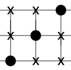
Previously in chapter A.4.6 we have used three CX gates to make a circuit equivalent in function to a single swap gate. It's a good idea to review it before the next task, which uses three CCX gates to make a Fredkin gate.
Please
Exercise
Using three CCX gates, create a circuit with the same function as a Fredkin gate with the control ball in the middle.
Expand by moving mouse over the exercise or by clicking
In the section on CCX gates, we noted that there are three different types of CCX gates: If you don't remember the difference between these, you should spend some time refreshing your memory on CCX gates back in chapter A.4.5. Since there are only three options for each step, you can quite easily try out all possible combinations. To speed up the testing, you can choose an input that distinguishes the desired Fredkin gate from all other Fredkin gates. This is related to the question before the exercise. Finally, you must of course verify all inputs, because one input will not distinguish the desired Fredkin gate from all other gates, even if it at least excludes the wrong kind of Fredkin gate.
A.5.6 Inverse gates
We have seen in the past that many gates are such that when two identical gates are placed in series, their function is negated. Recall the gates we have been through and answer the question below.
Please
Try it for yourself
Repeat the operation of the previous gates. Try each one by putting the same gate one after the other.
Expand by moving mouse over the exercise or by clicking
A gate that cancels the operation of a given gate is called its inverse gate. A gate can be its own inverse gate, but it can also be the case that the inverse gate is another gate. In any case, it follows from the mathematical structure of quantum theory that every quantum gate has an inverse gate. From this we can conclude that a circuit of quantum gates can be reversed, that is, a combination of gates can be found that reverses the action of the circuit.
In the following exercise, the brown box is an unknown gate. Combine the gates we know and find a combination that cancels out the unknown gate. This means that the output of input 0 should be 0 and input 1 should be 1.
Please
Exercise
Find a combination of gates that cancels the operation of an unknown gate.
Expand by moving mouse over the exercise or by clicking
Here the unknown gate gives 50 % probability for 0 an 1 If i add 2 X gates, the probablity remains the same as per simulator. the same is true if i add 2 H gates. but when the answer is saved, it says there is wrong probability for answer 0, which is wrong as per the output probability table.
—I need some help here. I am not understanding what is expected here. I tried with the finnish version too, even if there is no change in output probability the answer is not accepted.
As said above, find a combination that cancels out the unknown gate. This means that the output of input 0 should be 0 and input 1 should be 1. You have not found the correct combination yet.
—For ordinary gates, the inverse gate is found as we described, i.e. by searching for a combination of gates where the output is the same as the input for all the different inputs. For quantum gates, however, this is not enough. This is because the measurement does not reveal everything about the quantum state, and the gate may appear to have been canceled even if it has not restored the state to its initial state. An inverse gate for a given gate is a gate that cancels the effect of a gate even if they are in between other gates.
We have recently observed in chapter A.5.3 that two H gates in sequence do not have an effect on the input. Consequently, we can state that the output must be the same as the input, when a qubit is affected by a gate and its inverse gate surrounded by H gates.
Please
Try it yourself
Put your solution to the previous problem after the gate labelled '?'. Will the output be the same as the input?
Expand by moving mouse over the exercise or by clicking
The conclusion is that for quantum gates, the inverse gate must also be tested between the other gates. The combination of gates you found earlier is not a inverse gate of the unknown gate, as it does not negate the unknown gate between the H gates. It should be emphasized that when we talk about an unknown gate and its inverse gate, it is not necessarily any of the gates we named earlier. For example, a gate can be a combination of two gates.
It can be shown that for a single qubit, it is sufficient to consider gates without other gates and between two H gates. For a single qubit, the inverse gate is therefore a gate where the function of given gate is cancelled by all inputs
without other gates, and
between two H gates.
The figure below illustrates the two situations. It is essential that the green gate, which represents the inverse gate, is the same in both cases. The inverse gate can be a combination of several basic gates and is therefore depicted as a longer bar in the figure.
In both of these cases, the input must pass through unchanged -- the green gate is then the inverse gate of the unknown gate.
Let's return to our previous exercise. The inverse gate candidate we've found for the unknown gate satisfies condition (1), but not condition (2). We have more searching to do.
Please
Exercise
Find a combination of gates that cancels the unknown gate (1) so that there is nothing at steps 1 and 7 and (2) so that the H gates are at steps 1 and 7. <strong>Use the same combination of gates in both cases</strong> and place them between steps 3-6.
Expand by moving mouse over the exercise or by clicking
Here also the probability remains the same for any gate combination, but when the answer is saved it says there are wrong probabilities.
—Here also the output probability has not changed, but the answer is not accepted. I am may be not understanding what is expected here.
—Finally, let's recall that once the measurement is done, the calculation cannot be reversed back to the input. Quantum computation is reversible for quantum gates, but the last step, measurement, is not a reversible event.
A.5.7 The Z gate
Let us get familiar with one more quantum gate.
Please
Try it yourself
The Z gate is a quantum gate. Explore how it works.
Expand by moving mouse over the exercise or by clicking
As we noted in the section on inverse gates, the full function of quantum gates is not reflected in the changes to the initial states and . This is because a quantum gate can somehow change the superposition states without changing the states and at all.
Please
Try it yourself
Examine the operation of the Z gate when it is between other gates. The circuit has an XZX, i.e. a Z gate between two X gates. Try replacing the X gates with other gates. With another qubit you can compare how the gates work without the Z gate.
Expand by moving mouse over the exercise or by clicking
Then recall the definition of an inverse gate and use the previous quantum gate simulator to find the inverse gate for the Z gate. Be sure to test the combination without other gates and between the H gates.
Please
Exercise
Using the CZ gate and H gates, make a circuit with the same function as a single CX gate, where the X gate affects the q[0] qubit.
Expand by moving mouse over the exercise or by clicking
First you should remember how the CX gate works. Go back to the simulator and make yourself a table of the inputs and outputs. For instance, the input 00 gives the output 00 and the input 11 gives output 01. What about inputs 01 and 10?
As we have stated in a previous exercise, the "Z gate acts between two ----- gates like ----- gate alone." If you don't remember what the missing words are, then repeat the earlier part of this section. This is an essential clue to solving the problem.
The Z gate is a phase gate. This means that it does not alter the states or , but instead it changes the superposition states between them. How phase gates operate is rather simple, but we need some maths to model them. We will delve into the mathematical descriptions of qubit states and quantum gates in part B of the ABCs of Quantum Computing. That is where we will explain the operation of the Z gate in a detailed, exact manner.
A.5.8 The Quantum Computer
Gate computing is a model for a device that processes information - a computer. The reason we have gone through gate computing is that we need to have some definition of a normal computer before we can start thinking about more specialised computers. At this point, it should be mentioned that gate computing is only one of models that have been developed for information processing.

Correspondingly, quantum gate computing is a model for a device that processes quantum information. Naturally, such a device can then be called a quantum computer. A quantum computer takes a string of bits as input and outputs a string of bits, just like a regular computer. At the beginning of the processing, the bit string is written into the states of the quantum system. This way, the information is in the form of quantum information and can be processed by quantum gates. Finally, the measurement transforms the quantum information back into ordinary information, i.e. a bit string. In our exercises, this setup should have become clear to you.

Quantum gate computing as such is a rather abstract model for a quantum computer. From a more practical point of view, a quantum computer is something a little different. One can think of the device that performs the gate computation as the computer processor and the device that performs the quantum gate computation as the quantum processor. A quantum computer must have both kinds of processors, as well as some other components. In addition, there must be a program written for the quantum computer and a programming language suitable for its use.

Quantum physics allows one to process qubits in a way that is not possible for bits. We've previously explored the H gate, SX gate and Z gate, which cannot be performed on a bit. From this wider scope opened up by quantum physics comes the expectation of faster computation. With more options for basic operations, one can try to come up with new ways to compute something. However, using the quantum computer in a useful way is by no means straightforward. The quantum computer needs special quantum algorithms that make appropriate use of the new possibilities opened up by quantum physics. The quantum computer is therefore not a magic bullet that will immediately make all computation faster than supercomputers. It will probably only speed up the solution of certain types of computational problems.

Building a quantum processor is difficult. The single biggest reason is that quantum systems are susceptible to noise and interference. When there is too much noise, a quantum system is no better than a system that follows classical physics. So noise destroys the quantum properties of the system. In quantum physics, the time for which a quantum system retains its quantum properties is called coherence time. The phenomenon or event in which quantum properties are lost is called decoherence.

Going further into the requirements for a quantum processor, a good starting point is DiVincenzo's criteria for a quantum processor. They are a kind of checklist for the quantum processor builder of what needs to be in place. DiVincenzo's criteria are as follows:
- A scalable number of qubits. Scalability means that qubits can be added as needed. Typically, the number of qubits needed increases as the difficulty of the computational problem increases. Qubits are also needed for error correction. In the exercises of this course we have done very simple operations and the number of qubits has therefore been small.
- The ability to initialize the qubits used in the computation, i.e. to prepare them repeatedly in the initial state. In terms of the computation it is important that the qubits are in a known initial state at the beginning. It must be possible to return to the same state each time the computation is to be repeated. In a quantum gate computation, the initial state is usually the state in which each qubit is in the state .
- A sufficiently long coherence time. There is no specific threshold for the coherence time, but its adequacy is proportional to the speed of processing. The qubits must be able to perform the desired processing during the coherence time. In quantum gate computing, processing corresponds to the execution of gates.
- A universal set of quantum gates. A quantum gate set is said to be universal if it can be used to perform any quantum gate, or at least to approximate as precisely as desired. This means that a universal quantum gate set allows the implementation of any quantum algorithm. It can be shown that by combining quantum gates of one and two qubits, all other quantum gates can be implemented.
- Measuring qubits. Measurement is an essential part of quantum computing, since the final result of the computation is the bit string obtained from the measurement. The information carried by quantum systems cannot be read without measurement. The measurement process must be reliable and repeatable.

Depending on the physical implementation of the quantum processor, some gates are native, i.e. those that can be executed directly. Other gates are constructed as combinations of native gates. Due to the limited coherence time, it is desirable to try to perform the desired information processing using as small a number of gates as possible. However, this is complicated further by the fact that the execution time of native gates may also differ. Regardless, changing a circuit into a different circuit that performs the same processing is important for designing the execution of a quantum algorithm. In previous exercises, you have been able to find alternative implementations for certain circuits. For example, in chapter A.4.6 we saw that a swap gate can be built using CX gates.
A.6 Practice exercises
This chapter will be open to registered students of the course, when all earlier exercises are completed.
This chapter will open when you have completed all the previous exercises. In this chapter, you can review and practise what you have learned using a quantum gate simulator. The exercises may require several attempts.
A.7 Concluding remarks
This chapter will open to registered students of the course, when all exercises have been completed.
This chapter will open once you have answered all the questions and completed all the tasks. You can check Performances for questions and exercises still to be done.
List of quantum gates
The blue is for quantum gates that also work for bits. The violet is for quantum gates that only work for qubits.
Three qubit gates
- CCX gate = Toffoli gate
- Fredkin gate = controlled swap gate
Please
Kokeile itse
Here you can test the function of different quantum gates.
Expand by moving mouse over the exercise or by clicking
Please
Please
These are the current permissions for this document; please modify if needed. You can always modify these permissions from the manage page.
Writing a note in the margin is called commenting in TIM. It is worth making commenting an active part of your learning. Here's how to do it:
Note! Even if you write a comment for everyone, your name will not appear in it. You are welcome to share your thoughts with others.
If you have moved the editing menu to the left of the block, click on the block and the letter C (Comment) will appear on the right, click on the letter C