Agenda for week 6: Relativistic quantum mechanics
Learning goals for this week:
- General Lorentz invariance
- Why Schrödinger equation is not Lorentz invariant
- Relativistic extensions: Klein-Gordon equation and Dirac equation
- Dirac equation: spinor solutions (interpretation in the next lecture)
Reading assignment:
Notes for week 6: Relativistic quantum mechanics
More details:
- Tuominen, Secs 8.1, 8.2 (see also Secs 8.6, 8.7)
- Bransden & Joachain, Secs 15.1-15.4
- Sakurai & Napolitano, Secs 8.1 and 8.2
Preliminary exercises,
Do these during/after reading the assignment work. Will be discussed in class April 20th.
- Assume a Lorentz invariant form of a dynamical equation for the wave function
 , of the form
  = (-i\hbar c \vec \alpha \cdot \nabla
+ \beta mc^2) \psi(t,\vec r),") where
where  and
and  do not necessarily commute between each other. Requiring that
 ") also satisfies the Klein-Gordon equation, find the constraints (algebra) for
also satisfies the Klein-Gordon equation, find the constraints (algebra) for  and .
and .
- Taking the Dirac representation of
 check, for at least 2 different pairs
  that they satisfy the Clifford algebra relation.
- Check that for any constant 2-component vector
 , the following is a solution of the positive energy Dirac equation for a plane wave in the Dirac representation:
  = N(\mathbf p) \begin{pmatrix} \chi \\ \frac{\mathbf p\cdot\boldsymbol{\sigma}}{E_{\mathbf p}+m} \chi
\end{pmatrix},")
Homework exercises, week 6
Will be discussed in the tutorial session on Thursday April 22nd. Return a scanned pdf with your solution by Friday April 23rd, at 9 pm using the form below. Then check and grade your solution with the help of the model solutions and resubmit your graded solutions by Tuesday April 27th at 9 am.
Using the Klein-Gordon equation, show that the continuity equation
 , with four-current
 \Psi\right)") , holds.
, holds.Prove that the Klein-Gordon equation for a free particle is invariant under the transformation
 \mapsto \psi_c(t,{\bf x})=\hat C \psi(t,{\bf x})
\equiv \psi^*(t,{\bf x})") which describes charge conjugation. It relates the negative-energy solutions
which describes charge conjugation. It relates the negative-energy solutions  of the Klein-Gordon equation, that have no physical meaning individually, to the function
  that describes positive-energy states. The wavefunction
  \equiv \psi^*(t,{\bf x})") can be interpreted as the wavefunction of the antiparticle.
can be interpreted as the wavefunction of the antiparticle.Verify that if the function
is an eigenfunction of any of the operators  ,
,  ,
,  ,
,  , then the corresponding charge-conjugated function
  is also an eigenfunction. What is the relation between the corresponding charge-conjugated eigenvalues?
Show that the Lorentz boost into
 -direction,
  transforms the wave function by
  \mapsto \psi'(x') = S\psi(x)") with
with  .
.Remember that in general we parametrize the Hilbert space representation of a rotation by an angle
 around an axis
  with
with  by
by  where the operators
  are the rotation generators. What is the generator (for 4-component spinors) of a rotation around the
  axis in the Dirac representation? Is the spinor with
  an eigenvector of this generator, i.e. an eigenstate of the -component of spin?
Klein tunneling.
Prove that in 1+1 dimensions the (2)
 -matrices can be taken to have a representation in terms of Pauli matrices as
  , and
, and  .
.Write the 1D Dirac equation for a particle in a purely scalar potential (i.e.
\neq 0, \vec{A}=0") ), with the above choice for
), with the above choice for  and
and  . You can add the scalar potential by replacing
 ") in the Dirac equation.
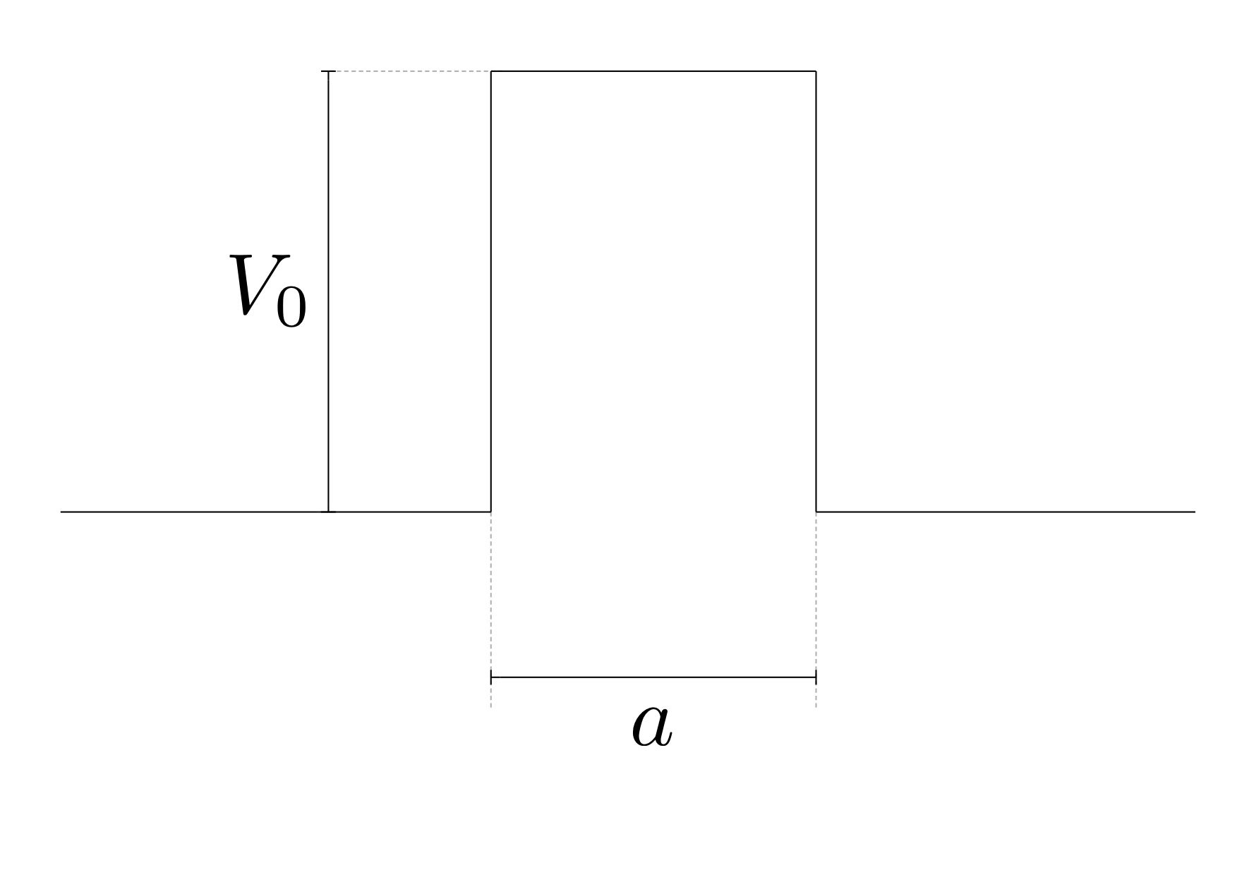
in the Dirac equation.Calculate the transmission probability for an electron scattering off a square potential barrier in 1D (see figure). Discuss in detail the case
 .
.
The Dirac equation for massless particles (in two-dimensional space) describes the behaviour of electrons in graphene, where traces of Klein tunneling have been observed, see N. Stander, B. Huard and D. Goldhaber-Gordon, Phys. Rev. Lett. 102, 026807 (2009) and A.F. Young and P. Kim, Nature Phys. 5, 222 (2009).
Solutions are here.
Exercise points (filled by TA)
Please
Notes for week 6: Relativistic quantum mechanics
The basic postulates of special relativity are: (i) the laws of nature are identical (invariant) in all inertial frames of reference, and (ii) the speed of light is same for all such frames. A consequence of these postulates is that there is no strict distinction between time and space, but that space and time dimensions appear different for observers moving at different speeds.
The Schrödinger equation is clearly incompatible with the special relativity: it is of the first order in time derivative, but of the second order in spatial derivatives. Our task in this part of the course is to find a relativistic generalization(s) of the Schrödinger equation.
To accomplish this, let us first remind ourselves of the mathematical formalism of special relativity. For a more detailed description of special relativity, see David Tong's lecture notes.
Elements of special relativity
In Minkowski space, one considers space and time coordinates together, as one four-vector  :
: ^{\intercal},") where
where  is the speed of light and
  is the Lorentz index. Strictly speaking, is the
  th component of the vector . Often, however, refers to the whole vector. From the context, it should be clear what one means.
We use greek letters to denote the Lorentz indices ( ). Roman letters are used to denote the spatial indices, (
 ).
).
The location of the indices is important: , with an upper index, is a contravariant vector. Correspondingly,  , with a lower index, is a covariant vector. In relativistic algebra, the difference between the two types of vectors is in how they transform in change of basis; covariant vectors change along the change of basis, whereas contravariant vectors change in an inverse way. Mathematically, contravariant vectors are elements of a vector space
  (i.e. vectors), and covariant vectors are elements of the dual space
  (i.e. dual vectors).
Metric tensor
We can lower the indices with the covariant metric tensor  ;
;  \equiv g_{\mu\nu} = g_{\nu\mu},") so that with every contravariant four-vector
so that with every contravariant four-vector  , we associate a covariant four-vector
  Above, we introduced the Einstein's summation convention, in which the repeated Lorentz indices are summed over. The notation is called Einstein notation.
With the above metric tensor, the components of the contravariant/covariant vectors are related by:  and
and  .
.
Similarly, we can lower an index in any higher order tensor  :
: 
Sometimes we have the opposite situation: we have a covariant vector  and we would like to find the corresponding contravariant vector. This can be done with the contravariant metric tensor
  :
:  We want this definition to be in harmony with the definition
  . Thus
  Since this is true for every vector,
  must be an identity in the sense that
  We conclude that the covariant and contravariant metric tensor are the inverses of each other (in the matrix sense)
  where the second step follows because in this case is its own inverse. The last step is only valid in the usual
  coordinate system, not for curved (such as spherical, cylindrical etc) coordinates or for a curved space-time.
We also note that due to the symmetry of the metric tensor ( ), it is not important which index we raise:
  For a general tensor,
  .
.
Inner product
As the name metric tensor suggests, we use  to define an inner product, which gives a notion of frame independent distance between two points in the Minkowski space:
  Separating the temporal and spatial parts, the Minkowski inner product is
  where the dot product between the spatial vectors is the usual Euclidean inner product. Notice the minus sign!
Convention note: here we are using the "mostly minus" or "west coast" metric, which is commonly used in particle physics. In general relativity and cosmology one uses the "mostly plus" or "east coast" metric ") , where the scalar product is
, where the scalar product is  .
.
Lorentz tranformations
A linear coordinate transformation is a real-valued 4x4 matrix  such that
  Here are the coordinates in the original coordinate system and
  are the coordinates after the transformation. The transformation can also be expressed as a derivative between the coordinates in transformed and original coordinate systems:
Lorentz transformations are defined as coordinate transformations which leave the inner product between four-vectors invariant, i.e.  for all and
  . These transformations form a group, known as the Lorentz group. Without reference to the vectors and , the condition which defines the Lorentz group is
By contracting both sides with  , we obtain
  so
so ^\mu}_\nu") is the matrix inverse of
is the matrix inverse of  , by which we mean that we can write the above equation in terms of matrix multiplication as
  The matrices are not defined systematically with regard to upper/lower indices; the components of are
  , whereas the components of are
  . From this equation we see that the matrix has the inverse
 ^\intercal,") which can be written in terms of the components as
which can be written in terms of the components as ^\mu{}_\nu \equiv [\Lambda^{-1}]_{\mu\nu} = [(g \Lambda g)^\intercal]_{\mu\nu}= [g \Lambda g]_{\nu\mu} = [g]_{\nu\alpha} [\Lambda]_{\alpha\beta} [g]_{\beta\mu} = g_{\nu\alpha} \Lambda^\alpha{}_\beta g^{\beta\mu} = \Lambda_\nu{}^\mu.")
We now show that the full Lorentz group divides into four distinct parts. The determinant taken from both sides of the above equation is ^2 \det g.") So we find that
So we find that  . As these are the only two allowed values, the determinant cannot be smoothly deformed from 1 to -1. These sets of transformations are thus in some sense disjoint from each other.
Consider then the  -component of the above equation:
 ^2 - \sum_{i=1}^3 ({\Lambda^i}_0)^2.") As is a real matrix, the sum of squares is positive and we find that
As is a real matrix, the sum of squares is positive and we find that ^2 \geq 1") . This can be satisfied either with
. This can be satisfied either with  or with
  . The latter transformation inverts time.
The group of all Lorentz transformations divides into four connected components:
 and . These are the proper Lorentz transformations. The simplest example is the identity transformation
  .
. and . Example:
 \rightarrow (-x^0,\mathbf x)") , i.e. inversion of time.
, i.e. inversion of time.- and . Example:
\rightarrow (x^0,-\mathbf x)") , i.e. inversion of space.
, i.e. inversion of space. - and . Example:
\rightarrow (-x^0,-\mathbf x)") , i.e. inversion of both time and space.
, i.e. inversion of both time and space.
In the following, unless stated otherwise, by Lorentz transformations we mean the proper transformations, which do not invert time (time reversal transformation) or space (parity transformations).
Proper rotations
Pure rotations form a subgroup of the Lorentz group. They are represented by the matrices ,") where
where ") is a rotation matrix. For example, a rotation of around the z-axis is given by a Lorentz transformation
is a rotation matrix. For example, a rotation of around the z-axis is given by a Lorentz transformation .")
Let us check that the four-vector inner product is invariant under rotations. The action on a coordinate four-vector is .") The inner product between four-vectors is:
The inner product between four-vectors is: ^\intercal (R\mathbf{y})\\
&= x^0 y^0-\mathbf{x}^\intercal R^\intercal R \mathbf y\\
&= x^0 y^0-\mathbf{x}^\intercal \mathbf y = x\cdot y,
\end{align*}") where we used the fact that for proper rotations
where we used the fact that for proper rotations  . Also
  and
and  , so this is indeed a proper Lorentz transformation.
Lorentz boosts
Apart from rotations, the other basic type of Lorentz transformation is a boost, a transformation to a frame moving at velocity  relative to the original frame. Let
  and
and  be two inertial frames such that at
  their origin and the coordinate axes coincide. Let us then assume that moves with a velocity
  relative to . On a course of special relativity we have learned that the coordinates in the two frames are related by
 \\
x' = \gamma(x-vt)\\
y' = y\\
z' = z,
\end{cases}") where
where  . The transformation between the two frames is represented by the matrix
 ") which can, like the rotation above, be verified to satisfy the conditions of a proper Lorentz transformation. Sometimes it is useful to parametrize the boost by so called rapidity
which can, like the rotation above, be verified to satisfy the conditions of a proper Lorentz transformation. Sometimes it is useful to parametrize the boost by so called rapidity ") . The above transformation then looks like
. The above transformation then looks like 
The rest of the Lorentz transformations can be generated as a combination of boosts and rotations. The larger symmetry group which also includes space-time translations  is known as the Poincare group.
Transformations of contravariant and covariant vectors
Above, we defined that the contravariant vectors transform as 
By using the metric tensor to manipulate the location of indices, we can prove that covariant vectors transform inversely under Lorentz transformations: ^\nu{}_\mu x_\nu.
\end{aligned}") The example below shows geometrically why the covariant vector transforms in an inverse way. It also shows mathematically what we mean by a transformation.
The example below shows geometrically why the covariant vector transforms in an inverse way. It also shows mathematically what we mean by a transformation.
Here we try to make the difference between contravariant and covariant vectors more concrete by using 2D rotations as an example. A transformation between two coordinate systems in physics translates to a basis transformation in linear algebra. The transformation is passive, which means that physically nothing changes, but that we adopt a different way of describing the situation. The alternative to a passive transformation would be an active transformation, which would correspond to e.g. physically rotating some object in a fixed coordinate system. Active tranformations are useful in the description of rotating bodies. Mathematically, there is no difference between the kinds of coordinate transformations, the difference is only in the interpretation of the mathematics.
Also, the difference between contravariant and covariant vectors is not particular to Minkowski space, but exists in any vector space. For an illustration, it is then enough to consider vectors on a plane where the only proper transformations between the orthonormal bases are rotations. Let us assume that we have two bases, ") and
and ") , where
, where  is obtained by rotating the basis vectors of by angle (see figure below):
 \begin{pmatrix} \cos\theta \\ -\sin\theta\end{pmatrix},\\
\hat e_2' &= \hat e_1 \sin\theta + \hat e_2\cos\theta = (\hat e_1, \hat e_2)\begin{pmatrix} \sin\theta \\ \cos\theta\end{pmatrix},
\end{aligned}") where we chose to represent the basis vectors as row vectors. The above two equations can be combined into a single matrix equation
where we chose to represent the basis vectors as row vectors. The above two equations can be combined into a single matrix equation  = (\hat e_1, \hat e_2)\begin{pmatrix} \cos\theta & \sin\theta\\ -\sin\theta & \phantom{+}\cos\theta\end{pmatrix} = (\hat e_1, \hat e_2) R^{-1},") which we would write in the covariant notation as
which we would write in the covariant notation as ^\nu{}_\mu\hat e_\nu") . Here
. Here  is a rotation matrix for a rotation of angle to positive direction. The transformation for the basis is a covariant transformation.
 -- (0,0);
\draw [<->,thick, blue] (0,2.5) node (yaxis) [above] {$\hat{e}_2$}
|- (2.5,0) node (xaxis) [right] {$\hat{e}_1$};
\node at (2.5*0.5,{2.5*sqrt(1-0.5^2)+0.15}) {$\hat{e}'_2$};
\node at ({2.5*sqrt(1-0.5^2)+0.15},-2.5*0.5) {$\hat{e}'_1$};
\draw [<->,thick, red] (2.5*0.5,{2.5*sqrt(1-0.5^2)}) node (yprimeaxis) {}
-- (0,0) -- ({2.5*sqrt(1-0.5^2)},-2.5*0.5) node (xprimeaxis) {};
\draw [->](0.7,0) arc(0:asin(-0.48):0.7) node[midway,right] {$\theta$};
\draw[->] (0,0.7) arc (90:90+asin(-0.48):0.7) node[midway,above] {$\theta$};
\draw[dashed] (yaxis |- xprimeaxis) node[left] {$-\sin\theta$}
-| (xaxis -| xprimeaxis) node[above] {$\cos\theta$};
\draw[dashed] (yaxis |- yprimeaxis) node[left] {$\cos\theta$}
-| (xaxis -| yprimeaxis) node[below] {$\sin\theta$};
\end{tikzpicture}")
Let us now define a vector which has components ^\intercal") in the basis (see the figure below):
in the basis (see the figure below): \begin{pmatrix} x^1 \\ x^2\end{pmatrix} = \hat e_\mu x^\mu") The vector
The vector  itself is independent of the choice of basis, but its coordinates
 ^\intercal") do depend on it. In the rotated basis , is expressed as
do depend on it. In the rotated basis , is expressed as \begin{pmatrix} x'^1 \\ x'^2\end{pmatrix} = \hat e'_\mu x'^\mu.") Equating the expressions for in bases and , and using the basis transformation law
Equating the expressions for in bases and , and using the basis transformation law = (\hat e_1, \hat e_2) R^{-1}") , we find that the coordinates transform as:
, we find that the coordinates transform as:  We call this a contravariant transformation, since it transforms against (contra-varies) the basis transformation.
 -- (0,0);
\draw [<->,thick, blue] (0,2.5) node (yaxis) [above] {$\hat{e}_2$}
|- (2.5,0) node (xaxis) [right] {$\hat{e}_1$};
\draw [<->,thick, red] (2.5*0.5,{2.5*sqrt(1-0.5^2)}) node (yprimeaxis) [above] {$\hat{e}'_2$}
-- (0,0) -- ({2.5*sqrt(1-0.5^2)},-2.5*0.5) node (xprimeaxis) [right] {$\hat{e}'_1$};
\draw [->](0.7,0) arc(0:asin(-0.48):0.7) node[midway,right] {$\theta$};
\draw[->] (0,0.7) arc (90:90+asin(-0.48):0.7) node[midway,above] {$\theta$};
\coordinate (c) at (2,1);
\coordinate (yprimeaxis) at ({(1+sqrt(1-0.5^2))*0.5},{(1+sqrt(1-0.5^2))*sqrt(1-0.5^2)});
\coordinate (xprimeaxis) at ({(-0.5+2*sqrt(1-0.5^2))*sqrt(1-0.5^2)},{-(-0.5+2*sqrt(1-0.5^2))*0.5});
\draw[dashed, blue] (yaxis |- c) node[left] {$x^2$}
-| (xaxis -| c) node[below] {$x^1$};
\draw[dashed,red] (yprimeaxis) node[left] {$x'^2$} -- (c) -- (xprimeaxis) node[below] {$x'^1$};
\draw [->, very thick] (0,0) -- (c) node[above right] {$\vec{x}$};
\end{tikzpicture}")
When we say that something transforms as a co/contravariant vector, we are abusing the terminology a bit. To be precise, we should say that it transforms like the coordinates of a co/contravariant vector.
Transformations of fields
Fields add another layer of complexity to transformations. Instead of a single scalar, vector or a tensor, we have a function over spacetime, so we have to transform both the field components and its argument (coordinates).
For concreteness, let us consider a vector field ") , which associates with each point
, which associates with each point  some vector
  = \hat e_\mu A^\mu(\vec x) = \hat e'_\mu A'^\mu(\vec x).") Here and
Here and  are coordinate-independent vectors and and are their coordinates in the basis
 ") . and
. and  are the coordinates of the same vectors in some other basis
 ") . For illustration, see the collapsible box above.
. For illustration, see the collapsible box above.
In the coordinate basis we write the above field as \equiv A^\mu(\hat e_\nu x^\nu) = A^\mu(\vec x),") where is the coordinate vector
where is the coordinate vector  . We omit the Lorentz index in the coordinate, since it is not useful to contract the argument e.g. with denoting the vector component of the field. In the coordinate basis we define similarly
  \equiv A'^\mu(\hat e'_\nu x'^\nu) = A'^\mu(\vec x).")
Now  , so the transformation rule for both the field components and its argument becomes
  &= A'^\mu(\vec x) = \Lambda^\mu{}_\nu A^\nu(\vec x)\\
&= \Lambda^\mu{}_\nu A^\nu(x) = \Lambda^\mu{}_\nu A^\nu(\Lambda^{-1} x').
\end{aligned}") On the first line we transform the vector field components (
On the first line we transform the vector field components ( ) and on the second line the coordinates (in ) and
  (in ) are related to each other.
We can write the above transformation law in a concise form  \rightarrow A'^\mu(x') = \Lambda^\mu{}_\nu A^\nu(x).") The above was for a contravariant vector field. For a scalar field we only transform the coordinate:
The above was for a contravariant vector field. For a scalar field we only transform the coordinate: \rightarrow \phi'(x') = \phi(x),") so that
so that  = \phi(\Lambda^{-1} x)") . In addition to scalars, vectors and tensors, a quantum theory admits also another kind of geometric entity: a spinor, which has its own transformation law. Spinors are discussed below.
. In addition to scalars, vectors and tensors, a quantum theory admits also another kind of geometric entity: a spinor, which has its own transformation law. Spinors are discussed below.
Partial derivatives
Let us define a partial derivative with respect to the components of a contravariant vector : 
= \left( \frac 1 c \frac {\partial}{\partial t},\nabla\right),") which acts on as
which acts on as  How does
  transform under Lorentz transformations? From the requirement
  for the transformed derivative, it can be verified that it transforms as a covariant vector, just as the notation suggests:
 ^\nu{}_\mu \partial_\nu.")
Similarly, we define a partial derivative with respect to a covariant vector: ^\intercal,") where the extra minus sign is required to cancel the minus signs in the defition of
where the extra minus sign is required to cancel the minus signs in the defition of  in order to have
  This derivative transforms as a contravariant vector:
Note: Be careful with the signs! Here, no minus signs appear:  Unlike here, where we do get a minus sign:
Four-momentum
Let us consider the relativistic generalization of momentum for a particle moving at velocity in the frame . From the Noether's theorem we learn that energy is the conserved quantity associated with the time translations, whereas momentum is the conserved quantity associated with the spatial translations. Thus we can assume that the relativistic generalization of momentum, four-momentum, has the form ,") but we do not know immediately the expressions for
but we do not know immediately the expressions for  and
and  .
.
However, we do know that the particle is at rest in the frame moving at velocity . In that frame the particle has no 3-momentum and thus we know that the 4-momentum is of the form .") The fact that we put a mass into the
The fact that we put a mass into the  component follows from dimensional analysis. Here we also require that
  , since a massless particle does not have a rest frame. To find the four-momentum in the frame , we make Lorentz boost from to . (Do this as an exercise!) The result is
  = m\gamma \mqty(c\\\mathbf{v}),")
The square of 4-momentum is a Lorentz invariant quantity ^2-|\mathbf p|^2.") In the rest frame, the energy is positive, so we find the relativistic dispersion of a free particle with mass
In the rest frame, the energy is positive, so we find the relativistic dispersion of a free particle with mass  :
:  A proper generalization of the Schrödinger equation should reproduce this dispersion.
Klein-Gordon equation
Note: From now on, we work in natural units  .
.
Recall how for a nonrelativistic system the Schrödinger equation }{\partial t} = \hat H \psi(\mathbf{x},t),") could be obtained from a classical Hamiltonian
could be obtained from a classical Hamiltonian =\frac{|\mathbf p|^2}{2m} +V(\mathbf{x})") by replacing and
by replacing and  by operators which obey the canonical commutation relations. The form of the Schrödinger equation in position representation suggests that we effectively did the replacements
  and
and  .
.
If we try to do the same replacement for the relativistic dispersion  , we fail. Even if we manage to interpret the square root operator
  meaningfully (e.g. by Fourier transform or series expansion), we end up with a complicated nonlocal operator.
If, instead, we start from the square of the above expression,  , we avoid such problems. We make the replacements
  and
and  and apply the resulting operator on a scalar field
 ") to obtain the Klein-Gordon equation
to obtain the Klein-Gordon equation \psi(\mathbf{x},t) = 0,") which can be written in Einstein notation as
which can be written in Einstein notation as \psi(\mathbf{x},t) = 0.") Klein-Gordon equation is clearly Lorentz invariant. So far everything is good. As we are attempting to generalize Schrödinger equation, we hope to be able interpret as a wavefunction of a particle.
Klein-Gordon equation is clearly Lorentz invariant. So far everything is good. As we are attempting to generalize Schrödinger equation, we hope to be able interpret as a wavefunction of a particle.
Like the Schrödinger equation, the Klein-Gordon equation has plane-wave solutions:  = \mathcal N e^{-i p\cdot x} = \mathcal N e^{-i (E t-\mathbf{p}\cdot\mathbf{x}) }.") Let us fix the momentum to some value and solve for the energy of this solution. Substituting the above into the Klein-Gordon equation, we find
Let us fix the momentum to some value and solve for the energy of this solution. Substituting the above into the Klein-Gordon equation, we find \psi_{\mathbf p}(\mathbf{x},t) = \left( -E^2 + |\mathbf p|^2 + m^2\right)\psi_{\mathbf{p}}(\mathbf{x},t) = 0,") which has two solutions:
which has two solutions:  . The positive energy solution is what we expected, but what are we to make of the negative energy solution?
It turns out the negative energy solutions make the theory unstable. The energy of a particle is not bounded from below, which means that there is no ground state. If we were to add a perturbation (e.g. potentials), they would couple the negative and positive energy states, and the particle could transition to lower and lower energy states.
The negative energies also force us to abandon the hope of interpreting as a wavefunction. As with the non-relativistic treatment, one obtains the continuity equation for the probability 4-current from the Klein-Gordon equation and its complex conjugate: =\frac{i}{2m}\left( \psi^*\partial^\mu\psi -(\partial^\mu\psi^*)\psi \right).") The "probability density"
The "probability density"  for a plane-wave solution is
  which is negative if
  . The conclusion is that we cannot interpret as a probability density and thus is not a wavefunction.
It turns out that the classical Klein-Gordon equation can be used to derive a relativistic quantum field theory for spin-0 particles (e.g. pion or Higgs boson), but the quantization requires either the use of path integrals or the full machinery of canonical quantization (not that this would be very hard; we already did it for the electromagnetic field in the QED part of the course). Luckily, there is another equation which we can quantize with the above simple procedure, the Dirac equation, which turns out to describe electrons and other spin-½ particles.
Dirac equation
Dirac ansatz
In 1928, Paul Dirac developed a new field equation for spin-½ particles. For the (very readable) original article, see here. Dirac's motivation was to derive an equation which would not have the problems of the Klein-Gordon equation. The negative energy states in Klein-Gordon equation seem to stem from the fact that it is of the second order in time derivative, thus his idea was to search for a first order equation both in  and
and  , by first assuming a general ansatz
 }{\partial t} = H_D \psi(\mathbf{x},t)
%= (-i c\boldsymbol{\alpha}\cdot \nabla+\beta m c^2)\psi(\mathbf{x},t),
= (-i \boldsymbol{\alpha}\cdot \nabla+\beta m )\psi(\mathbf{x},t),") where the four initially unknown quantities
where the four initially unknown quantities  and commute with
  (i.e. they do not depend on ) but not with each other. As groups can typically be represented by matrices, we can assume that
  and are N×N matrices, where the dimension N is as of yet unknown. In order to have a compatible structure with the matrices,
 ") must then be a (complex) N×1 column vector.
must then be a (complex) N×1 column vector.
Dirac then required that the field should also satisfy the Klein-Gordon equation, to guarantee that the relativistic dispersion relation  holds for the solutions of the equation:
(-i\boldsymbol{\alpha}\cdot \mathbf \nabla+\beta m)\psi\\") Moving towards the covariant formulation, we write the above as
Moving towards the covariant formulation, we write the above as  m \partial_i + \beta^2 m^2 \right]\psi = 0") The Klein-Gordon equation, on the hand, can be written as
The Klein-Gordon equation, on the hand, can be written as \psi = 0,") Comparing the two equations above term by term, we find that Dirac's ansatz satisfies the Klein-Gordon equation if and only if
Comparing the two equations above term by term, we find that Dirac's ansatz satisfies the Klein-Gordon equation if and only if  Furthermore, we require that the Hamiltonian
  is Hermitian:
  . In the exercises it will be shown that and are hermitean, traceless, even-dimensional, mutually anticommuting matrices. The lowest dimensional matrices that can represent them are 4×4 matrices.
The above requirements do not fix and uniquely, so we have some freedom in choosing their representation. There are a few common choices. We take the Dirac-Pauli representation (or basis), with which the non-relativistic limit is particularly simple,  where
where  's are the Pauli matrices and
  is the 2×2 identity matrix. The other commonly used choices for and matrices go by the names Weyl representation and Majorana representation.
Probability current
Because the Hamiltonian is Hermitian, the probability amplitude  = \psi(\mathbf{x},t)^\dagger\psi(\mathbf{x},t)") is conserved:
is conserved:  &= (\partial_t \psi)^\dagger\psi + \psi^\dagger (\partial_t \psi)\\
&= -(iH_D \psi)^\dagger\psi + \psi^\dagger (i H_D \psi)\\
&= \left[(\nabla \psi^\dagger\cdot\boldsymbol{\alpha})\psi + \psi^\dagger(\boldsymbol{\alpha}\cdot\nabla \psi)\right]\\
&= \nabla\cdot (\psi^\dagger \boldsymbol{\alpha}\,\psi) \equiv \nabla\cdot\mathbf j,
\end{aligned}") Also, by definition,
Also, by definition, \geq0") . In this sense we have improved from the Klein-Gordon equation.
. In this sense we have improved from the Klein-Gordon equation.
Now you should be able to go back and do Question 1 in the preliminary exercises
Covariant equation of motion
To formulate the Dirac equation in a covariant form, we multiply both sides of the equation by and define a new set of matrices  which have the anticommutation relations
  defining a Clifford algebra. Because of this algebraic structure, the -matrices have a lot of useful properties. However, we do not discuss these in detail, but we just give one identity that is used in derivations below:
 ^\dagger=\gamma^0\gamma^\mu\gamma^0.") This identity is independent of the choice of the representation.
This identity is independent of the choice of the representation.
In terms of -matrices, the Dirac equation becomes  \psi(x) = 0.")
In particle physics, the Feynman slash notation  is often used, so that we obtain an even more condensed form
  \psi = 0.")
Note that even if the -matrices carry the Lorentz index of the partial derivative, they do not transform as contravariant vectors. We have defined them as constant matrices so they do not change at all in Lorentz transformations. Next, we show how the wavefunction ") should transform so that the Dirac equation would be Lorentz invariant.
should transform so that the Dirac equation would be Lorentz invariant.
Note: The defined above is like any other one-particle Hamiltonian: We can replace the non-relativistic Hamiltonian with it and do calculations as before. The only caveat is that its eigenenergy spectrum is not bounded from below, as discussed below. This problem can be addressed only in a many-body formulation.
Properties of -matrices
Any product of -matrices can be expressed as a linear combination of the following sixteen matrices:  where
where  and
and  . Within some representation, any complex 4×4 matrix
  can be written as a linear combination of the above matrices:
  , where
  are (representations of) the 16 matrices above. The usefulness of this matrix basis is that the bilinears
  (
( is defined below) have simple properties under Lorentz transformations:
  \Lambda^\mu{}_\nu \bar\psi\gamma^5 \gamma^\nu\psi && \text{contravariant pseudovector}\\
\bar\psi'\gamma^5\psi' &= \det(\Lambda)\bar\psi\gamma^5\psi && \text{pseudoscalar}
\end{aligned}") The quantities with the prefix "pseudo" change sign on parity transformation.
The quantities with the prefix "pseudo" change sign on parity transformation.
Different representations of the -matrices
There are three commonly used representations for matrices. In each representation, some particular property is diagonal or otherwise simple.
- In Dirac(-Pauli) basis the upper and lower spinor components correspond to particle and antiparticle solutions, respectively, in the non-relativistic limit.

- In Weyl (chiral) basis, the chiral operator
 is diagonal:
- Majorana basis is chosen so that all the matrices are purely imaginary:
 where
where  is the charge conjugation operator, which is typically of interest for Majorana fermions. In this basis, it acts in a simple way:
 ^\intercal") .
.
Choosing the above  matrix representation for the -matrices means that the eigenvectors satisfying the Dirac equation are spinors of the form
  = \begin{pmatrix} \psi_0(x) \\ \psi_1(x) \\ \psi_2(x) \\ \psi_3(x) \end{pmatrix}.") Below we discuss the form of the eigenfunctions of the Dirac equation. But let us first check how such spinors transform under Lorentz transformations. These 4-component spinors can be built from two 2-component spinors (see the section about Weyl fermions below), and are sometimes called bi-spinors.
Below we discuss the form of the eigenfunctions of the Dirac equation. But let us first check how such spinors transform under Lorentz transformations. These 4-component spinors can be built from two 2-component spinors (see the section about Weyl fermions below), and are sometimes called bi-spinors.
Lorentz transformation of spinors
We now derive the transformation law for , by assuming that the form of the Dirac equation is invariant under Lorentz transformations. We can assume that transforms linearly under Lorentz transformations:  \rightarrow \psi'(x') = S(\Lambda)\psi(x),") where
where ") is a 4×4 matrix representation of the Lorentz transformation . We know how the partial derivative transforms:
is a 4×4 matrix representation of the Lorentz transformation . We know how the partial derivative transforms: ^\nu{}_\mu \partial_\nu") The Dirac equation
The Dirac equation \psi(x)=0") transforms into
transforms into \psi'(x') &= (i\gamma^\mu(\Lambda^{-1})^\nu{}_\mu \partial_\nu-m)S(\Lambda)\psi(x)\\
&= S(\Lambda)\left[iS(\Lambda^{-1})(\Lambda^{-1})^\mu{}_\nu\gamma^\nu S(\Lambda) \partial_\mu -m\right]\psi(x),
\end{aligned}") which has, apart from the factor on the left, the same form as the original equation if obeys the equation
which has, apart from the factor on the left, the same form as the original equation if obeys the equation (\Lambda^{-1})^\mu{}_\nu \gamma^\nu S(\Lambda) = \gamma^\mu") , which is equivalent to
, which is equivalent to \gamma^\mu S(\Lambda) = \Lambda^\mu{}_\nu \gamma^\nu.") This equation gives the connection between a Lorentz transformation and its spinor representation . If is known, it is possible to compute .
This equation gives the connection between a Lorentz transformation and its spinor representation . If is known, it is possible to compute .
You might recall from non-relativistic QM that the Pauli matrices obey a similar equation:  where is a rotation matrix for rotation of angle around the axis
  and
and ") is the corresponding unitary transformation for spinors.
is the corresponding unitary transformation for spinors.
Let us define the commutator of two -matrices:  For example, a Lorentz boost of rapidity
  to x direction,
 ^\mu{}_\nu =
\begin{pmatrix}
\cosh\xi & -\sinh\xi & 0 & 0\\-\sinh\xi & \cosh\xi & 0 & 0\\ 0 & 0 & 1 &0\\ 0& 0& 0& 1
\end{pmatrix},") is represented by a spinor transformation (left here as an exercise)
is represented by a spinor transformation (left here as an exercise)  = \exp(-\xi \sigma^{01}/4) = \cosh\frac \xi 2-\gamma^0\gamma^1 \sinh\frac \xi 2,") and a rotation of angle around z-axis (or equivalently: on xy-plane, which is what the indices of
and a rotation of angle around z-axis (or equivalently: on xy-plane, which is what the indices of  refer to) is represented by
  = \exp(\theta\sigma^{12}/4)=
\begin{pmatrix}
\exp(-i\theta\sigma_3/2) & 0\\
0 & \exp(-i\theta\sigma_3/2)
\end{pmatrix},") which contains two copies of the same non-relativistic rotation. The above examples suggest that a spinor rotation is unitary,
which contains two copies of the same non-relativistic rotation. The above examples suggest that a spinor rotation is unitary,  = S(\Lambda_2)^\dagger") , but a spinor boost is not:
, but a spinor boost is not: \neq S(\Lambda_1)^\dagger") .
.
To find the inverse transformation ^{-1}=S(\Lambda^{-1})") we take a Hermitian conjugate of the equation relating and :
we take a Hermitian conjugate of the equation relating and : ^\dagger(\gamma^\nu)^\dagger S(\Lambda^{-1})^\dagger = \Lambda^\mu{}_\nu (\gamma^\mu)^\dagger.") Then we use the identity
Then we use the identity ^\dagger=\gamma_0\gamma^\nu\gamma_0") and multiply from both sides with
and multiply from both sides with  :
: ^\dagger\gamma_0\gamma^\nu \gamma_0 S(\Lambda^{-1})^\dagger\gamma_0 = \Lambda^\mu{}_\nu \gamma^\mu.") Comparison with the original equation suggests that
Comparison with the original equation suggests that  = \gamma^0 S(\Lambda)^\dagger\gamma^0.") That this is indeed the inverse of can be verified from the general solution
That this is indeed the inverse of can be verified from the general solution =\exp(\frac 1 2 \omega_{\mu\nu}\sigma^{\mu\nu})") , where
, where  is a real antisymmetric matrix which parametrizes the Lorentz transformations.
Lorentz transformation of spinors =\exp\left(\frac 1 2 \omega_{\mu\nu}\sigma^{\mu\nu}\right),") where is a real antisymmetric matrix which parametrizes the Lorentz transformations and
where is a real antisymmetric matrix which parametrizes the Lorentz transformations and  + different conventions for
  and factors
  ,
,  in different sources
Dirac adjoint and relativistic scalars
The 4×1 column vectors act as the kets of the Dirac equation. Given a ket , what is the corresponding bra, i.e. the 1×4 row vector, which would allow us to calculate expectation values by sandwiching operators between bras and kets? A natural first guess would the hermitean conjugate  . However, this does not work since, e.g. the bilinear
  is not a Lorentz invariant scalar:
 ^\dagger S(\Lambda) \psi \neq \psi^\dagger\psi,") because, as we saw above, is not unitary if is a Lorentz boost.
because, as we saw above, is not unitary if is a Lorentz boost.
The solution is to define a Dirac adjoint  for which the bilinear
  is Lorentz invariant.
The necessicity of defining the adjoint  can be traced back to the Clifford algebra and the
 ") signature of the metric tensor, which forces the eigenvalues of some of the -matrices to be imaginary. Because of this, all the matrices cannot be unitary.
signature of the metric tensor, which forces the eigenvalues of some of the -matrices to be imaginary. Because of this, all the matrices cannot be unitary.
Sandwiched between the spinors, the -matrices effectively transform according to their Lorentz indices. For example, the quantity  transforms as a Lorentz vector,
  transforms as a rank-2 contravariant tensor and so on.
Dirac Lagrangian
One of the most important scalars which we can construct from the Dirac bilinears is the Lagrangian density \psi.") The Euler-Lagrange equations of motion obtained by variation of this Lagrangian should correspond to the Dirac equation. As is complex, the number of degrees of freedom are twice the number of components of ; thus we can treat as independent of and vary by and independently. Variation by
The Euler-Lagrange equations of motion obtained by variation of this Lagrangian should correspond to the Dirac equation. As is complex, the number of degrees of freedom are twice the number of components of ; thus we can treat as independent of and vary by and independently. Variation by  - \frac{\delta \mathcal L}{\delta\psi}=0,") gives
gives  which is the adjoint equation. The Dirac equation can be recovered by conjugation and multiplication by . Variation by ,
  - \frac{\delta \mathcal L}{\delta\bar\psi}=0,") gives the Dirac equation more directly.
gives the Dirac equation more directly.
From the Lagrangian density one can construct the action  and start building the path-integral formulation (not on this course though). The great benefit of the path-integral formulation is that we do not have choose a distinguished time-axis as in the Hamiltonian formulation, and the explicit relativistic covariance can be preserved.
Now you should be able to go back and do Question 2 in the preliminary exercises
Plane wave solutions
Let us find the plane wave solutions for the Dirac equation with an ansatz  = u(\mathbf p) e^{-i p\cdot x} = u(\mathbf p) e^{-i(E t-\mathbf p\cdot \mathbf x)},") where
where ") is a 4-component spinor. Let us see if we still have the negative energy solutions. By the above substitution the Dirac equation becomes
is a 4-component spinor. Let us see if we still have the negative energy solutions. By the above substitution the Dirac equation becomes  = (\boldsymbol{\alpha}\cdot\mathbf p+\beta m) u(\mathbf p).") The above can we written in block matrix form as
The above can we written in block matrix form as \\
u_B(\mathbf p)
\end{pmatrix}
=0,") where
where  and
and  are 2-component spinors. The eigenvalues satisfy the condition
 =0") .
.
The determinant condition is explicitly ^2 = (E^2 - |\mathbf p|^2- m^2)^2,
\end{aligned}") which has the solutions
which has the solutions  . Thus we did not cure the theory of the negative energy solutions. For convenience, we define a positive energy dispersion
  .
.
};
%Here the red parabloa is defined
\addplot [
domain=-5:5,
samples=100,
color=blue,
style=thick
]
{-sqrt(x^2+1)};
\end{axis}
\end{tikzpicture}")
Fig: Spectrum of the Dirac equation with a mass (solid line). The dashed line is the spectrum when  .
.
To gain understanding of the form of the solutions, set  . We find the solutions
  = N(0)\begin{pmatrix}
1\\0\\0\\0
\end{pmatrix},\quad
u_2(0) = N(0)\begin{pmatrix}
0\\1\\0\\0
\end{pmatrix},\quad
u_3(0) = N(0)\begin{pmatrix}
0\\0\\1\\0
\end{pmatrix},\quad
u_4(0) = N(0)\begin{pmatrix}
0\\0\\0\\1
\end{pmatrix},") where
where ") is a normalization constant. The particle is at rest, so its energy should be composed purely of the rest mass. Indeed, we find for the first solutions that
is a normalization constant. The particle is at rest, so its energy should be composed purely of the rest mass. Indeed, we find for the first solutions that  , which is positive, and for the last two
  , which is negative.
For  , the block-wise equation can be solved as
  = \begin{pmatrix} u_A(\mathbf p)\\u_B(\mathbf p) \end{pmatrix} = \begin{pmatrix} u_A(\mathbf p)\\ \frac{\mathbf p\cdot\boldsymbol{\sigma}}{E_{\mathbf p}+m} u_A(\mathbf p)\end{pmatrix},") where is a 2-component spinor which can be chosen freely, reflecting the spin degree of freedom. We choose as a basis the spin-up and spin-down states in the -direction:
where is a 2-component spinor which can be chosen freely, reflecting the spin degree of freedom. We choose as a basis the spin-up and spin-down states in the -direction: }_A(\mathbf p)=N(\mathbf p)\chi_+ = N(\mathbf p)\begin{pmatrix}1\\0\end{pmatrix},\quad u^{(2)}_A(\mathbf p)=N(\mathbf p)\chi_- = N(\mathbf p)\begin{pmatrix}0\\1\end{pmatrix}.") The above choice of basis is just a parametrization of the upper component. In general, the lower component has a different direction of spin and the bi-spinor is not an eigenstate of spin.
The above choice of basis is just a parametrization of the upper component. In general, the lower component has a different direction of spin and the bi-spinor is not an eigenstate of spin.
For , the block-wise equation can be solved as  = \begin{pmatrix} u_A(\mathbf p)\\u_B(\mathbf p) \end{pmatrix} = \begin{pmatrix} -\frac{\mathbf p\cdot\boldsymbol{\sigma}}{E_{\mathbf p}+m} u_B(\mathbf p)\\ u_B(\mathbf p)\end{pmatrix},") where is again arbitrary 2-component spinor. As above, we use for it the basis
where is again arbitrary 2-component spinor. As above, we use for it the basis  (multiplied by a normalization constant).
For given momentum , we have four linearly independent solutions  = N(\mathbf p)\begin{pmatrix} 1\\0\\ \frac{p_z}{E_{\mathbf p}+m} \\ \frac{p_x+ip_y}{E_{\mathbf p}+m}\end{pmatrix},\quad
u^2(\mathbf p) =N(\mathbf p)\begin{pmatrix} 0 \\ 1 \\ \frac{p_x-ip_y}{E_{\mathbf p}+m} \\ -\frac{p_z}{E_{\mathbf p}+m}\end{pmatrix},")
 = N(\mathbf p)\begin{pmatrix} -\frac{p_z}{E_{\mathbf p}+m} \\ -\frac{p_x+ip_y}{E_{\mathbf p}+m} \\ 1 \\ 0\end{pmatrix},\quad
u^4(\mathbf p) = N(\mathbf p)\begin{pmatrix} -\frac{p_x-ip_y}{E_{\mathbf p}+m} \\ \frac{p_z}{E_{\mathbf p}+m}\\ 0 \\ 1\end{pmatrix},") which have the energies
which have the energies  and
and  . The normalization
 ") can be chosen in different ways, depending on the context. Different normalizations are defined in the collapsible box below, along with identities related to
can be chosen in different ways, depending on the context. Different normalizations are defined in the collapsible box below, along with identities related to  's.
's.
The general solution of the Dirac equation can be written as  = \int\frac{{\rm d}^3\mathbf p}{(2\pi)^3} \left[ \sum_{s=1,2} a_s(\mathbf p)u^s(\mathbf p) e^{-i(E_{\mathbf p}t-\mathbf p\cdot\mathbf x)} + \sum_{s=3,4} a_s(\mathbf p)u^s(\mathbf p) e^{-i(-E_{\mathbf p}t-\mathbf p\cdot\mathbf x)}\right],") where
where ") 's are complex number coefficients. The solution can be written in a more symmetric way by defining the antiparticle spinors
's are complex number coefficients. The solution can be written in a more symmetric way by defining the antiparticle spinors  = u^4(-\mathbf p) = N(\mathbf p)\begin{pmatrix} \frac{\boldsymbol{\sigma}\cdot\mathbf p}{E_{\mathbf p}+m}\chi_- \\ \chi_- \end{pmatrix},\\
v^2(\mathbf p) = u^3(-\mathbf p) = N(\mathbf p)\begin{pmatrix} \frac{\boldsymbol{\sigma}\cdot\mathbf p}{E_{\mathbf p}+m}\chi_+ \\ \chi_+ \end{pmatrix},
\end{aligned}") and making the change of variables
and making the change of variables  on the second sum:
  = \int\frac{{\rm d}^3\mathbf p}{(2\pi)^3} \sum_{s=1,2} \left[ a_s(\mathbf p)u^s(\mathbf p) e^{-i p\cdot x} + b_s^*(\mathbf p)v^s(\mathbf p) e^{i p\cdot x}\right],") where
where ") is the four-momentum of the positive energy solution, and the coefficients are
is the four-momentum of the positive energy solution, and the coefficients are  = a_{4/3}(-\mathbf p)") .
.
Stueckelberg-Feynman interpretation
Since (-t)}=e^{-i E_{\mathbf p}t}") , we can interpret negative energy solutions in two mathematically equivalent ways;
, we can interpret negative energy solutions in two mathematically equivalent ways;
- as negative-energy particles going backward in time, or
- as positive-energy antiparticles going forward in time.
Both viewpoints can be used. This is the Stueckelberg-Feynman interpretation. It is used in Feynman diagrams, in which particles are depicted as arrows along the time direction, and antiparticles are depicted as arrows opposite to the time direction.
;
\coordinate[below right=of e1] (aux1);
\coordinate[above right=of aux1,label=right:$\gamma$] (e2);
\coordinate[below=1.25cm of aux1] (aux2);
\coordinate[below left=of aux2,label=left:$e^+$] (e3);
\coordinate[below right=of aux2,label=right:$\gamma$] (e4);
\draw[postaction={decorate},
decoration={markings,mark=at position .5 with {\arrow{triangle 45}}}] (e1) -- (aux1);
\draw[postaction={decorate},
decoration={markings,mark=at position .5 with {\arrow{triangle 45}}}] (aux2) -- (e3);
\draw[postaction={decorate},
decoration={markings,mark=at position .6 with {\arrow{triangle 45}}}] (aux1) -- (aux2);
\draw[decorate, draw=black, decoration={coil,aspect=0}] (aux1) -- (e2);
\draw[decorate, draw=black, decoration={coil,aspect=0}] (aux2) -- (e4);
%\draw[decorate, draw=black,
% decoration={coil,aspect=0}] (aux1) -- node[label=right:$\mkern-65muV_2(\vec q)\mkern30mu\vec q$] {} (aux2);
\draw[->] (0.4,0) --+ (0.7,-0.5) node[midway, above right] {$\mathbf p_1$};
\draw[->] (0.4,-3.3) --+ (0.7,0.5) node[midway, below right] {$\mathbf p_2$};
\end{tikzpicture}")
Fig: Example of a Feynman diagram, which depicts electron-positron annihilation and a creation of two photons. The positive time direction is from left to right. With the Stueckelberg-Feynman interpretation, the directed particle-antiparticle lines are always continuous. In this diagram, two photons are needed to satisfy both energy and momentum conservation laws.
Spinor normalization and identities
Now you should be able to go back and do Question 3 in the preliminary exercises
There are a few common conventions for the normalization of the spinors. They can be written in a unified way as  = \sqrt{\frac{E_{\mathbf p}+m}{\lambda}},") where
where  is a normalization parameter. Let us put a particle in a box of volume , and compute the total charge of a plane wave
  = \frac{1}{\sqrt{V}}u^s(\mathbf p)e^{-ip\cdot x}") :
: \psi(\mathbf x,t) = q\, u^s(\mathbf x)^\dagger u^s(\mathbf x)\\
&= q N(\mathbf p)^2 \frac {2E_{\mathbf p}}{E_{\mathbf p}+m}= q\frac{2E_{\mathbf p}}{\lambda} \equiv q\gamma_N,
\end{aligned}") where
where  is the charge of one particle. The field is not yet quantized, so its charge can take any value.
 is the covariant normalization. In this case
  . This normalization compensates for the shrinkage of in Lorentz boosts. With this normalization,
  in the rest frame.
 is a very often used normalization in high-energy physics. In this case
  , and in the rest frame
  .
. normalizes the wave functions to unity. This is the usual normalization we use when doing quantum mechanics non-covariantly within the Hamiltonian formalism.
Below, the identities which involve adjoint spinors are more naturally given in covariant or high-energy normalization, whereas the identities involving Hermitian conjugate spinors are simpler in the normalization .
The plane wave spinors obey the following identities:
- Orthogonality:
^\dagger u^s(\mathbf p) &= \frac{2E_{\mathbf p}}{\lambda}\delta_{rs},\\
v^r(\mathbf p)^\dagger v^s(\mathbf p) &= \frac{2E_{\mathbf p}}{\lambda}\delta_{rs},\\
u^r(\mathbf p)^\dagger v^s(-\mathbf p) &= v^r(-\mathbf p)^\dagger u^s(\mathbf p) = 0,
\end{aligned}") where
where  .
. - For conjugate spinors,
 \equiv u^\dagger(\mathbf p)\gamma^0") , one has the identities
, one has the identities  u^s(\mathbf p) &= \frac{2m}{\lambda}\delta_{rs},\\
\bar v^r(\mathbf p)v^s(\mathbf p) &= -\frac{2m}{\lambda}\delta_{rs},\\
\bar u^r(\mathbf p)v^s(\mathbf p) &= \bar v^r(\mathbf p)u^s(\mathbf p) = 0,
\end{aligned}") where
where  and no sum over
  is implied. These relations are Lorentz-invariant.
 - -matrices inserted inside the Dirac bilinear give
 \gamma^\mu u^s(\mathbf p) &= \frac{2p^\mu}{\lambda}\delta_{rs},\\
\bar v^r(\mathbf p) \gamma^\mu v^s(\mathbf p) &= -\frac{2p^\mu}{\lambda}\delta_{rs}.
\end{aligned}")
- One can define projection operators (up to a constant) to particle and antiparticle states, respectively:
 \bar u^s(\mathbf p) &= \frac{1}{\lambda}(p\mkern-8mu/+m),\\
\sum_{s=1,2} v^s(\mathbf p) \bar v^s(\mathbf p) &= \frac{1}{\lambda}(p\mkern-8mu/-m).
\end{aligned}") Note the order of the spinors, these are 4×4 matrix identities.
Note the order of the spinors, these are 4×4 matrix identities. - By subtracting the two projection operators from each other, a completeness relation (resolution of identity for states with momentum ) is obtained:
\bar u^s(\mathbf p)- v^s(\mathbf p)\bar v^s(\mathbf p)\right] = \frac{2m}{\lambda}1_4.") The above identity shows how the antiparticles are essential to the theory: without the antiparticle spinors one does not obtain a complete set of states and cannot write down a resolution of identity.
The above identity shows how the antiparticles are essential to the theory: without the antiparticle spinors one does not obtain a complete set of states and cannot write down a resolution of identity. - Non-covariant form of the resolution of identity is
 u^s(\mathbf p)^\dagger = \sum_{s=1,2}\left[ u^s(\mathbf p) u^s(\mathbf p)^\dagger + v^s(-\mathbf p) v^s(-\mathbf p)^\dagger\right]= \frac{2E_{\mathbf p}}{\lambda} 1_4.")
These are the current permissions for this document; please modify if needed. You can always modify these permissions from the manage page.