I. Feynman path integrals
Learning goals:
Main idea of posing the quantum mechanics axioms in terms of path integrals instead of the usual operator formalism
Path integrals for a single spinless particle moving in a one-dimensional system.
Harmonic oscillator propagator and the saddle point approximation
An alternative formulation of the dynamics in quantum mechanics is given by the path integrals. This formulation was developed by Richard Feynman and it is equivalent with the formulations discussed in Ch. III. The path integral approach is particularly important and useful for quantum field theories, especially for non-Abelian gauge-field theories, such as quantum chromodynamics exhibiting strong interactions, and the unified electroweak theory in the Standard model of particle physics. However, it is also used in several other branches of physics and even beyond physics for example in econophysics. In statistical mechanics it allows for a practical approach for treating stochastic phenomena (Feynman-Vernon approach).
Some historical references on this approach are
R.P. Feynman: Space-time approach to Non-Relativistic Quantum Mechanics
R.P. Feynman and F.L. Vernon: The theory of a general quantum system interacting with a linear dissipative system
Here, we limit the study to the perhaps simplest case of quantum mechanics of one spinless particle in a one-dimensional system. Let us start by reminding of the Schrödinger picture wave function, or the position representation of the state vector, \[\psi(x,t) \equiv {}_S\langle x|\psi(t)\rangle_S.\] It quantifies the probability amplitude for finding the particle at a certain location at a certain time. In what follows, we concentrate exclusively on the Schrödinger picture and therefore drop the subscript S.
The time evolution of a state in the Schrödinger picture can be written as \[|\psi(t)\rangle = \hat U(t,t_0) |\psi(t_0)\rangle.\] Then \[\begin{aligned} \psi(x'',t'')&=\langle x''|\psi(t'')\rangle = \langle x'' |\hat U(t'',t)\underbrace{ }_{\hat 1=\int_{-\infty}^\infty dx |x\rangle \langle x|} |\psi(t)\rangle\\ &=\int_{-\infty}^\infty dx \underbrace{\langle x''|\hat U(t'',t)|x\rangle}_{G(x'',t'';x,t)} \underbrace{\langle x | \psi(t)\rangle}_{\psi(x,t)}.\end{aligned}\] In other words, \[\psi(x'',t'')=\int_{-\infty}^\infty dx G(x'',t'';x,t) \psi(x,t),\] where the Feynman kernel or the propagator is \[G(x'',t'';x,t) \equiv \langle x''|\hat U(t'',t)|x\rangle.\] From above, we see that the "propagation" of the wave function, or the states, from \(t\) to \(t'\) is controlled by the function \(G(x'',t'';x,t)\).
Especially, if the particle is in an eigenstate \(|x'\rangle\) of \(\hat x\) (\(\hat x |x'\rangle = x'|x'\rangle\)) at the time \(t'\), the probability amplitude for finding the particle in a state \(|x''\rangle\) at time \(t''\) is given by the propagator: \[\begin{aligned} \psi(x'',t'')=\langle x''|\hat U(t'',t')|\psi(t')\rangle \overset{\psi(t')=|x'\rangle}{=}\langle x''|\hat U(t'',t')|x'\rangle = G(x'',t'';x',t').\end{aligned}\] In the following, let us assume that \(\hat H\) does not depend on time. Then, from Sec. III, \[\hat U(t,t_0)=e^{-\frac{i}{\hbar}(t-t_0) \hat H} = \hat U(t-t_0).\] and as a result, \[\boxed{G(x'',t'';x',t')=\langle x''|e^{-\frac{i}{\hbar} (t''-t') \hat H}|x'\rangle = G(x'',x',t''-t')}\] In the exercises, we will compute the propagator of a free particle (\(\hat H=\frac{\hat p^2}{2m}\)). It reads \[G_{\rm free}(x'',x';t''-t')=\sqrt{\frac{m}{2\pi i (t''-t')\hbar}} e^{\frac{i}{\hbar} \frac{m}{2(t''-t')} (x''-x')^2}. \] Below we see how this result is computed from the path integral.
Now, let us develop the path integral formulation for the propagator. We start from a single step: \[\begin{aligned} G(x'',t'';x,t)&\equiv \langle x''|e^{-\frac{i}{\hbar} \hat H (t''-t)} |x\rangle = \langle x''|e^{-\frac{i}{\hbar} \hat H (t''-t')} \underbrace{ }_{\hat 1} e^{-\frac{i}{\hbar} \hat H(t'-t)} |x\rangle\\ &=\int_{-\infty}^\infty dx' \langle x''|e^{-\frac{i}{\hbar} \hat H (t''-t')} |x'\rangle \langle x'| e^{-\frac{i}{\hbar} \hat H (t'-t)} |x\rangle \\ &=\int_{-\infty}^\infty dx' G(x'',t'';x',t') G(x',t';x,t).\end{aligned}\] Here we also inserted the resolution of unity \(\hat 1 = \int_{-\infty}^\infty dx |x\rangle \langle x|\). Although the equation as such holds for any set of times, assume here that \(t''>t'>t\).
The single propagator thus divides into two: The probability amplitude for finding the particle at a position \(x''\) at a time \(t''\), when it originally at time \(t\) was at a location \(x\), is given by multiplying the probability amplitudes for the particle to first move from \((x,t)\) to \((x',t')\) and then from \((x',t')\) to \((x'',t'')\), and summing (integrating) over all possible intermediate locations \(x'\). This is the basis of the path integral formulation.
Let us now repeat this procedure many times, so that the time interval \(t''-t\) gets split into \(N\) intervals of the same length \(\delta t=t_{i+1}-t_i\): \[t''-t=\underbrace{t''-t_{N-1}}_{\delta t_N} + \underbrace{t_{N-1}-t_{N-2}}_{\delta t_{N-1}} + t_{N-2} - \dots + \underbrace{t_2-t_1}_{\delta t_2} + \underbrace{t_1-t}_{\delta t_1}.\] Thus, \(t''-t=N \delta t\), in which \(N\rightarrow \infty\) and \(\delta t \rightarrow 0\).
The propagator now divides into pieces:
\[ G(x'',t'';x,t)=\langle x''| e^{-\frac{i}{\hbar} \hat H \delta t_N} e^{-\frac{i}{\hbar} \hat H \delta t_{N-1}} \cdots e^{-\frac{i}{\hbar} \hat H \delta t_1} |x\rangle. \] Let us now insert a resolution of unity of the form \[ \hat 1 = \int_{-\infty}^\infty dx_j |x_j\rangle \langle x_j| \] before each of the term of the form \(e^{-\frac{i}{\hbar} \hat H \delta t_j}\), \(j=1, \dots N\). We get \[ G(x'',t'';x,t)=\int_{-\infty}^\infty dx_N \cdots \int_{-\infty}^\infty dx_1 \underbrace{\langle x''|x_N\rangle}_{\delta(x''-x_N)} \langle x_N|e^{-\frac{i}{\hbar} \hat H \delta t_N}|x_{N-1}\rangle \cdots \langle x_1|e^{-\frac{i}{\hbar} \hat H \delta t_1}|x\rangle \] or \[\boxed{G(x'',t'';x,t)=\left[\prod_{i=1}^{N\rightarrow \infty} \int_{-\infty}^\infty dx_i G(x_i,t_i;x_{i-1},t_{i-1})\right]\delta(x''-x_N)} \] where \(x_0 = x\), \(t_0=t\), \(t_N=t''\), and \(t_i-t_{i-1}=\delta t\).
Graphically this looks as follows:

In other words, every possible path from \(x\) to \(x''\) is included!
Now suppose that \[\hat H=\frac{\hat p^2}{2m}+V(\hat x).\] Then \[e^{-\frac{i}{\hbar} \hat H \delta t} = e^{-\frac{i}{\hbar} [\frac{\hat p^2}{2m}+V(\hat x)] \delta t} = e^{\underbrace{-\frac{i}{\hbar} \frac{\hat p^2}{2m}\delta t}_{\hat A}\underbrace{-\frac{i}{\hbar}V(\hat x)\delta t}_{\hat B}}.\] Note that the operators \(\hat A\) and \(B\) do not usually commute: \([\hat A,\hat B]\neq 0\). Therefore, we have \[e^{\hat A+\hat B} = e^{\hat A} e^{\hat B} e^{-\frac{1}{2}[\hat A,\hat B]+\dots},\] where the "\(\dots\)" indicate higher-order commutators between \(\hat A\) and \(\hat B\). Now, note that \([\hat A,\hat B] = o((\delta t)^2)\) when \(N\rightarrow \infty\). Thus, we can use \[e^{-\frac{i}{\hbar} \hat H \delta t} = e^{-\frac{i}{\hbar} \frac{\hat p^2}{2m}\delta t}e^{-\frac{i}{\hbar}V(\hat x)\delta t} \underbrace{e^{o((\delta t)^2)}}_{1+o((\delta t)^2)}.\]
For the infinitesimal period \(\delta t\) we thus have the propagator \[\langle x_i |e^{-\frac{i}{\hbar} \hat H \delta t_i} |x_{i-1}\rangle \approx \langle x_i | e^{-\frac{i}{\hbar}\frac{\hat p^2}{2m} \delta t} \underbrace{ }_{\hat 1} e^{-\frac{i}{\hbar} V(\hat x) \delta t} |x_{i-1}\rangle, \] where we insert \(\hat 1 = \int_{-\infty}^\infty dp_{i-1} |p_{i-1}\rangle \langle p_{i-1}|.\)
It thus becomes \[ \langle x_i |e^{-\frac{i}{\hbar} \hat H \delta t_i} |x_{i-1}\rangle \approx \int dp_{i-1} \langle x_i | e^{-\frac{i}{\hbar}\frac{\hat p^2}{2m} \delta t} |p_{i-1}\rangle \langle p_{i-1}| e^{-\frac{i}{\hbar} V(\hat x) \delta t} |x_{i-1}\rangle. \] Now the operators operate on their eigenstates so we may replace \(\hat p\) by \(p_{i-1}\) and \(\hat x\) by \(x_{i-1}\). Now inserting \(\hat 1 = \int dp' |p'\rangle \langle p'|\) in front of the first exponential, and \(\hat 1=\int dx' |x'\rangle \langle x'|\) in front of the other, we get \[ \langle x_i |e^{-\frac{i}{\hbar} \hat H \delta t_i} |x_{i-1}\rangle \approx \int dp' dx' dp_{i-1} \langle x_i | p'\rangle \langle p'|e^{-\frac{i}{\hbar} \frac{p_{i-1}^2}{2m} \delta t} |p_{i-1}\rangle \langle p_{i-1}| x'\rangle \langle x'| e^{-\frac{i}{\hbar} V(x_{i-1}) \delta t} |x_{i-1}\rangle. \] Now, using the representation of the plane wave states, \(\langle x_i|p'\rangle = e^{\frac{i}{\hbar} x_i p'}/\sqrt{2\pi \hbar}\) and the fact that the matrix elements \(\langle p' |p_{i-1}\rangle = \delta(p'-p_{i-1})\) etc., we finally get this to the form \[ \langle x_i |e^{-\frac{i}{\hbar} \hat H \delta t_i} |x_{i-1}\rangle \approx \int \frac{dp_{i-1}}{2\pi \hbar} e^{\frac{i}{\hbar} \bigg[p_{i-1}(x_i-x_{i-1})-\delta t \underbrace{\left(\frac{p_{i-1}^2}{2m} + V(x_{i-1})\right)}_{H(p_{i-1},x_{i-1})}\bigg]}[1+o((\delta t)^2)]. \] Note that this form contains no operators, so the Hamiltonian in the remaining expression is classical.
Substitute this to the equation for the propagator. It becomes \[ G(x'',t'';x,t)=\left[\prod_{i=1}^N \int_{-\infty}^\infty dx_i G(x_i,t_i;x_{i-1},t_{i-1}) \right] \delta(x''-x_N) \\= \left(\prod_{i=1}^N \int_{-\infty}^\infty dx_i\right) \left(\prod_{i=0}^{N-1} \int_{-\infty}^\infty \frac{dp_i}{2\pi \hbar}\right) \delta(x_N-x'') \\\times e^{\frac{i}{\hbar} [p_{N-1} (x_N-x_{N-1})-\delta t H(p_{N-1},x_{N-1})]} \cdots e^{\frac{i}{\hbar} [p_{0} (x_1-x)-\delta t H(p_0,x)]} [1+o((\delta t)^2)]. \] Now use \(p_{j} (x_{j+1}-x_{j}) = \delta t p_{j} (x_{j+1}-x_{j})/\delta t\) so that we get \[ G(x'',t'';x,t)=\frac{1}{(2\pi \hbar)^N}\left[\prod_{i=1}^{N-1} \int_{-\infty}^\infty dx_i \int_{-\infty}^\infty dp_i\right]\int_{-\infty}^\infty dp_0 \\e^{\frac{i}{\hbar} \sum_{j=0}^{N-1} \delta t [p_j \frac{x_{j+1}-x_j}{\delta t} -H(p_j,x_j)]} [1+o((\delta t)^2)]. \] Note that in the limit \(\delta t \rightarrow 0\), the sum in the exponent becomes an integral.
We obtain \[\begin{split} G(x'',t'',x,t) \overset{N\rightarrow \infty}{=}& \frac{1}{(2\pi \hbar)^N} \left(\prod_{i=1}^{N-1} \int_{-\infty}^\infty dx_i \int_{-\infty}^\infty d p_i \right) \int_{-\infty}^\infty dp_0\\&\times e^{\frac{i}{\hbar} \int_{t}^{t''} dt'[p(t') \dot x(t')-H(p(t'),x(t'))]}\\ \equiv &\int_{x(t)=x}^{x(t'')=x''} [{\cal D}p] [{\cal D}x] e^{\frac{i}{\hbar} \int_{t}^{t''} dt' [p(t') \dot x(t') - H(p(t'),x(t'))]}. \end{split}\] This is the path integral representation of the propagator. The above formula also defines the sums over all path and momenta, \([{\cal D} p][{\cal D}x]\).
In the above expansion, the whole phase space (\(x\) and \(p\)) is integrated over. We can actually still do the integrals over momenta. For example, \[ \langle x_{i-1} | e^{-\frac{i}{\hbar} \hat H \delta t}|x_i\rangle = \int \frac{dp_i}{2\pi \hbar} e^{\frac{i}{\hbar}[p_i(x_{i+1}-x_i)-\delta t \frac{p_i^2}{2m} -\delta t V(x_i)]}\\ =\frac{1}{2\pi \hbar} e^{-\frac{i}{\hbar} \delta t V(x_i)} \int_{-\infty}^\infty d p_i e^{-i\alpha p_i^2 +i\beta p_i}, \] where \(\alpha=\frac{1}{\hbar} \frac{\delta t}{2m} > 0\) and \(\beta = \frac{1}{\hbar} p_i (x_{i+1}-x_i)\).
The exponent in the Gaussian integral is \[-i\alpha p_i^2+i\beta p_i = -i\alpha(p_i^2-\frac{\beta}{\alpha} p_i)=-i\alpha(p_i^2 - 2 \frac{\beta}{2\alpha} p_i + \frac{\beta^2}{4 \alpha^2}-\frac{\beta^2}{4\alpha^2}).\]
Hence \[ \int_{-\infty}^\infty dp_i e^{-i\alpha p_i^2 + i\beta p_i} = e^{i\frac{\beta^2}{4\alpha}} \int_{-\infty}^\infty dp_i e^{-i\alpha (p_i-\frac{\beta}{2\alpha})^2}\\= e^{i\frac{\beta^2}{4\alpha}} \int_{-\infty}^\infty d p_i' e^{-i\alpha p_i^2} = e^{i\frac{\beta^2}{4\alpha}} \sqrt{\frac{\pi}{i\alpha}}= \sqrt{\frac{\pi \hbar 2m}{i\delta t}} e^{\frac{i}{\hbar} \delta t \frac{m}{2} \left(\frac{x_{i+1}-x_i}{\delta t}\right)^2}. \]
The Gaussian integral can be found for example from https://en.wikipedia.org/wiki/Gaussian_integral.
The infinitesimal propagator is thus \[\langle x_{i+1} |e^{-\frac{i}{\hbar} \hat H \delta t} |x_i\rangle = \sqrt{\frac{m}{2\pi i \hbar \delta t}} e^{\frac{i}{\hbar} \delta t \frac{m}{2} \left(\frac{x_{i+1}-x_i}{\delta t}\right)^2 - \frac{i}{\hbar} \delta t V(x_i)}\] Substituting again this back in Eq. [eq:prop1] gives \[\begin{aligned} G(x'',t'';x,t)\overset{N\rightarrow \infty}{=}& \left(\prod_{i=1}^N \int_{-\infty}^\infty dx_i\right) \delta(x_N-x'') \left(\frac{m}{2\pi i \hbar \delta t}\right)^{N/2}\\&\times e^{\frac{i}{\hbar} \sum_{j=0}^{N-1} \delta t \left[\frac{m}{2} \left(\frac{x_{j+1}-x_j}{\delta t}\right)^2 - V(x_j)\right]}.\end{aligned}\] We hence get the Feynman path integral formulation of the propagator: \[\begin{split} G(x'',t'';x,t) =& \lim_{N\rightarrow \infty} \left(\frac{m}{2\pi i \hbar \delta t}\right)^{N/2} \left(\prod_{i=1}^N \int_{-\infty}^\infty dx_i\right)\\ &\times e^{\frac{i}{\hbar} \sum_{j=0}^{N-1} \delta t \left[\frac{m}{2} \left(\frac{x_{j+1}-x_j}{\delta t}\right)^2 - V(x_j)\right]}\\ \equiv& \int_{x(t)=x}^{x(t'')=x''} [{\cal D}x] e^{\frac{i}{\hbar} S(x'',t'';x,t)}. \end{split} \] Here the analogue of the classical action is \[S(x'',t'';x,t) \equiv \int_{t}^{t''} dt' L(x(t'),\dot x(t')).\] and the Lagrange function of the system is \[L(x(t),\dot x(t))\equiv \frac{m}{2} \dot x^2-V(x).\]
We thus arrived in a configuration (\(x\)) space path integral form of the propagator of the system \(\hat H=\frac{\hat p^2}{2m}+V(\hat x).\) The integration measure \({\cal D}x\) is defined with the above formula.
From here, we can see how quantum and classical mechanics differ in their behavior with respect to the path integral:
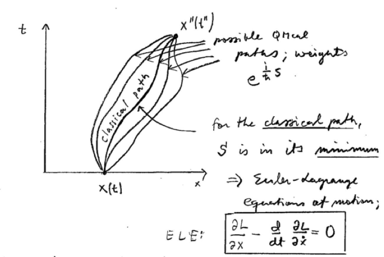
Let us look at the orders of magnitude, considering a classical free particle for which \(L(x,\dot x)=\frac{1}{2} m\dot x^2\). Then \[\frac{\partial L}{\partial x}=0;\quad \frac{\partial L}{\partial \dot x}=m \dot x\] The Euler-Lagrange equation hence yields \[\frac{\partial L}{\partial x}-\frac{d}{dt} \frac{\partial L}{d\dot x} = 0 \Rightarrow m\ddot x=0 \Rightarrow \dot x(t)=\dot x(t_0)=v_0.\] Then the classical action is \[S_{\rm cl}=\int_{t_0}^t dt' L(x,\dot x)=\int_{t_0}^t dt' \frac{1}{2} m \dot x^2 = \frac{1}{2} m v_0^2 (t-t_0).\] Let us put in some numbers corresponding to a macroscopic system, say \(m=2\) kg, \(v_0=1\) m/s, \(t-t_0=1\) s. In this case \[\frac{S_{\rm cl}}{\hbar} \approx \frac{1 {\rm Js}}{10^{-34} {\rm Js}} = 10^{34} \gg 1!\] Now, if \(S_{\rm cl}\) is not at its minimum, the weight \(e^{\frac{i}{\hbar} S}\) oscillates rapidly. The contributions from such oscillations thus average out, and only the classical path corresponding to \({\rm min}S_{\rm cl}\) is relevant in macroscopic systems.
For a quantum mechanical system, \(S/\hbar\) corresponding to different paths is not large (for example, \(m_e = 9\times 10^{-31}\) kg). Thus, in microscopic systems, many paths contribute, yielding the quantum effects.
In the Feynman path integral formulation of the propagator, Eq. [eq:feynmanpropagator], we can make the following observations:
The constant \(\left(\frac{m}{2\pi i \hbar \delta t}\right)^{N/2} \overset{N\rightarrow \infty}{\rightarrow} \infty^{\infty}\), but when computing physical quantities from the path integral, this constant cancels out. This means that the limit \(N\rightarrow \infty\) should usually be done last.
Obviously, the whole path integral does not converge even when \(N \rightarrow \infty\). We hence need further definitions, which correspond to certain boundary conditions and convergence factors \(i\epsilon\).
I.1 Free-particle propagator
In certain cases, the propagators can be solved exactly from the path integral. Such cases are
Free particle, \(L=\frac{1}{2} m \dot x^2\)
Harmonic oscillator, \(L=\frac{1}{2}m\dot x^2 - \frac{m}{2} \omega^2 x^2\)
Forced harmonic oscillator, \(L=\frac{1}{2}m\dot x^2 - \frac{m}{2} \omega^2 x^2+fx\).
Let us first look at the free-particle propagator. Now the path integral is, using \(V=0\) in Eq. [eq:feynmanpropagator] \[\begin{split} G(x'',t'';x,t) =& \lim_{N\rightarrow \infty} \left(\frac{m}{2\pi i \hbar \delta t}\right)^{N/2} \left(\prod_{i=1}^N \int_{-\infty}^\infty dx_i\right)\\ &\times e^{\frac{i}{\hbar} \sum_{j=0}^{N-1} \delta t \left[\frac{m}{2} \left(\frac{x_{j+1}-x_j}{\delta t}\right)^2\right]} \end{split} \] Now the \(\int_{-\infty}^\infty dx_i\)-integrals are all Gaussian, and can therefore be straightforwardly done (see exercises). In the end, one should notice that \(N\delta t=t''-t\). As a result, no \(N\) appears in the final result, given by Eq. [eq:freeparticlepropagator].
I.2 Semiclassical approximation of path integrals
Let us consider one possible way to treat the path integral, [eq:feynmanpropagator], the semiclassical approximation or the Gaussian approximation. This is probably the most often used approach for solving path integrals. In essence, the semiclassical approximation linearizes the system dynamics around some (classical) fixed point. For harmonic oscillators, which are linear systems (their average elongation is linearly proportional to the force), this becomes an exact treatment.
The basic idea here is to make an expansion with respect to the deviations from the classical paths \(x_{\rm CL}(t)\).
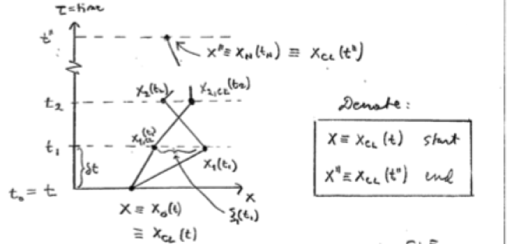
Let us hence write \[x(\tau)\equiv x_{\rm CL}(\tau) + \xi(\tau), \] where \(\xi(\tau)\) is a deviation from the classical path. Remember, in the path integral, the "path" denotes the positions \(x_1(t_1),x_2(t_2),\dots,x_N(t_N)\) over which the integral in Eq. [eq:feynmanpropagator] is taken. In particular, the end points at \(t=t_0\) and \(t=t_N\) are fixed to \(x=x_{\rm CL}(t=t_0)\) and \(x''=x_{\rm CL}(t_N=t'')\). In other words, the deviation satisfies at the end points \[\boxed{\xi(t=t_0)=0, \quad \xi(t''=t_N)=0}\]
Now, let us make a change of variables over which we integrate in Eq. [eq:feynmanpropagator]: \[x_i=x_{i,{\rm CL}}+\xi_i.\] Thus \[dx_i = \underbrace{dx_{i,{\rm CL}}}_{=0} + d \xi_i = d \xi_i,\] because the classical path is fixed. This means that the path integral measure over \(x(t)\) is the same as the one over \(\xi(t)\): \[[{\cal D} x] = [{\cal D} \xi]\] and the propagator is \[G(x'',t'';x,t) = \int_{\xi(t)=0}^{\xi(t'')=0} [{\cal D}\xi] e^{\frac{i}{\hbar} \int_t^{t''} dt' L[x_{\rm CL}(t')+\xi(t');\dot x_{\rm CL}(t')+\dot \xi(t')]}.\] Now let us assume that the major contribution to the integral comes from the paths that are close to \(x_{\rm CL}\), i.e., corresponding to small deviations \(\xi(t)\). This means that we can expand the exponent around \(\xi(\tau)=0\).
Let us start by expanding the Lagrange function to the second order in \(\xi\) and \(\dot \xi\). \[\begin{aligned} L(x=x_{\rm CL} + \xi;\dot x=\dot x_{\rm CL}+\dot \xi) =& \underbrace{L(x_{\rm CL}+\dot x_{\rm CL})}_{L_{\rm CL}} \\ &+\xi \frac{\partial L}{\partial x_{\rm CL}} + \dot \xi \frac{\partial L}{\partial \dot x_{\rm CL}}\\ &+\frac{1}{2} \xi^2 \frac{\partial^2 L}{\partial x_{\rm CL}^2} + \frac{1}{2} \dot \xi^2 \frac{\partial^2 L}{\partial \dot x_{\rm CL}^2} + \xi \dot \xi \frac{\partial^2 L}{\partial x_{\rm CL} \partial \dot x_{\rm CL}}\\ &+\underbrace{o(\xi^3,\dot \xi^3,\xi \dot \xi^2,\xi^2 \dot xi)}_{=o(\xi^3)},\end{aligned}\] where we use a short-hand notation \[\frac{\partial L}{\partial x_{\rm CL}} \equiv \frac{\partial L}{\partial x}|_{x=x_{\rm CL},\dot x=\dot x_{\rm CL}}, \quad \frac{\partial L}{\partial \dot x_{\rm CL}} \equiv \frac{\partial L}{\partial \dot x}|_{x=x_{\rm CL},\dot x=\dot x_{\rm CL}}.\]
For the action, this means \[\begin{aligned} S(x'',t'';x,t) =& \int_{t}^{t''} dt' L(x(t'),\dot x(t'))\\ &=\underbrace{\int_{t}^{t''} dt' L_{\rm cl}(t')}_{=S_{\rm cl}(x'',t'';x,t)}\\ &+\int_{t}^{t''} dt' [\xi \frac{\partial L}{\partial x_{\rm CL}} + \dot \xi \frac{\partial L}{\partial \dot x_{\rm CL}}]\\ &+\int_{t}^{t''} dt' [\frac{1}{2} \xi^2 \frac{\partial^2 L}{\partial x_{\rm CL}^2} + \frac{1}{2} \dot \xi^2 \frac{\partial^2 L}{\partial \dot x_{\rm CL}^2} + \xi \dot \xi \frac{\partial^2 L}{\partial x_{\rm CL} \partial \dot x_{\rm CL}}]\\ &+o(\xi^3).\end{aligned}\] Note that the linear terms in \(\xi\) vanish: \[\begin{aligned} \int_{t}^{t''} dt' [\xi \frac{\partial L}{\partial x_{\rm CL}} + \dot \xi \frac{\partial L}{\partial \dot x_{\rm CL}}] =& \int_t^{t''} dt' [\xi \frac{d}{dt'} \frac{\partial L}{\partial \dot x_{\rm CL}} + \dot \xi \frac{\partial L}{\partial \dot x_{\rm CL}}]\\ =& \underbrace{|_t^{t''} \xi \frac{\partial L}{\partial \dot x_{\rm CL}}}_{=0 \text{ since } \xi(t)=\xi(t'')=0} + \int_t^{t''} dt' [\underbrace{-\dot \xi \frac{\partial L}{\partial \dot \xi_{\rm CL}} + \dot \xi \frac{\partial L}{\partial \dot x_{\rm CL}}}_{=0}].\end{aligned}\] The first equality uses the Euler-Lagrange equation, \(\frac{\partial L}{\partial x_{\rm CL}}= \frac{d}{dt} \frac{\partial L}{\partial \dot x_{\rm CL}}\), and the second a partial integral to move the time derivative.
With this expansion, the action thus becomes \[\begin{split} S(x'',t'';x,t)=S_{\rm CL}(x'',t'';x,t) + \int_{t}^{t''} dt'[\frac{1}{2}\xi^2 \frac{\partial L}{\partial x_{\rm CL}^2} + \frac{1}{2} \dot \xi^2 \frac{\partial L}{\partial \dot x_{\rm CL}^2} + \xi \dot \xi \frac{\partial L}{\partial x_{\rm CL} \partial \dot x_{\rm CL}}] + o(\xi^3). \end{split}\] and the path integral becomes \[\begin{split} &G(x'',t'';x,t)=\int_0^0 [{\cal D}\xi] e^{\frac{i}{\hbar} S(x'',t'';x,t)}\\ =&e^{\frac{i}{\hbar} S_{\rm CL}(x'',t'';x,t)} \int_0^0 [{\cal D}\xi] e^{\frac{i}{\hbar} \int_{t}^{t''} dt'[\frac{1}{2}\xi^2 \frac{\partial L}{\partial x_{\rm CL}^2} + \frac{1}{2} \dot \xi^2 \frac{\partial L}{\partial \dot x_{\rm CL}^2} + \xi \dot \xi \frac{\partial L}{\partial x_{\rm CL} \partial \dot x_{\rm CL}}]}. \end{split} \] The above expression now expresses the main idea: the classical part \(S_{\rm CL}\) factorizes out of the path integral, and can thus be computed separately. For the remaining part, the path integral has to be performed using the discretized form in Eq. [eq:feynmanpropagator]. Let us do this using the harmonic oscillator as an example. The general case goes then very similarly.
I.3. Propagator of the harmonic oscillator
The Lagrange function for the harmonic oscillator is \[\boxed{L(x,\dot x)=\frac{1}{2} m \dot x^2-\frac{1}{2} m \omega^2 x^2}\] The derivatives needed for the action are \[\begin{aligned} \frac{\partial L}{\partial x} = -m\omega^2 x, \quad \frac{\partial^2 L}{\partial x^2} = -m\omega^2, \quad \frac{\partial^n L}{\partial x^n}=0, n>2\\ \frac{\partial L}{\partial \dot x} = m\dot x, \quad \frac{\partial^2 L}{\partial \dot x^2} = m, \quad \frac{\partial^n L}{\partial \dot x^n}=0, n>2\\ \frac{\partial^{n+m} L}{\partial x^n \partial^m \dot x}=0, \text{ for any $n,m \ge 1$}\end{aligned}\] Because the higher-order (than second) derivatives vanish, the semiclassical approximation gives the exact result for a harmonic oscillator!
Now, let us use these results to calculate the term in the deviation action, Eq. [eq:semiclassicalpi]: \[\frac{1}{2}\xi^2 \frac{\partial^2 L}{\partial x_{\rm CL}^2} + \frac{1}{2} \dot \xi^2 \frac{\partial^2 L}{\partial \dot x_{\rm CL}^2} + \xi \dot \xi \frac{\partial^2 L}{\partial x_{\rm CL} \partial \dot x_{\rm CL}}=-\frac{1}{2} m\omega^2 \xi^2 + \frac{1}{2} m \dot \xi^2.\] The discretized form of the action thus becomes (see Eq. [eq:feynmanpropagator]) \[\begin{aligned} \int_t^{t''}dt'[{ }] \overset{N\rightarrow \infty}{\leftarrow}& \sum_{j=0}^{N-1} \left[\frac{1}{2} m \underbrace{\left(\frac{\xi_{j+1}-\xi_j}{t_{j+1}-t_j}\right)^2}_{\dot \xi^2}-\frac{1}{2} m \omega^2 \xi_j^2\right]\delta t\\ =&\sum_{j=0}^{N-1} \left[\frac{m}{2\delta t} (\xi_{j+1}-\xi_j)^2 - \frac{\delta t}{2} m\omega^2 \xi_j^2\right].\end{aligned}\] Thus the discretized form of the path integral becomes \[\begin{split} G(x'',t'';x,t)=&e^{\frac{i}{\hbar} S_{\rm CL}(x'',t'';x,t)} \lim_{N\rightarrow \infty} \bigg\{\left(\frac{m}{2\pi i\hbar \delta t}\right)^{N/2} \prod_{i=1}^{N-1} \int_{-\infty}^\infty d\xi_i \\ &\times e^{\frac{i}{\hbar} \sum_{j=0}^{N-1} \left[\frac{m}{2\delta t} (\xi_{j+1}-\xi_j)^2-\frac{\delta t}{2} m\omega^2 \xi_j^2\right]}\bigg\} \end{split} \]
Here we used \([{\cal D} \xi]=[{\cal D} x]\) and the definition of \([{\cal D} x]\) from Eq. [eq:feynmanpropagator] with \(\xi_0=\xi_N=0\).
Now to proceed, we need to evaluate \(N-1 \rightarrow \infty\) (mixed) Gaussian integrals in a systematic way. The trick in this case is the write the sum in the exponent in a matrix form, \(\xi^T A \xi\), find the matrix \(A\), diagonalize it and then do the remaining separate Gaussian integrals. Let us see how this goes, as the method is useful also in general.
We want: \[ \sum_{j=0}^{N-1} [\frac{m}{2\delta t} (\xi_{j+1}-\xi_j)^2 - \frac{\delta t}{2} m\omega^2 \xi_j^2] \equiv \xi^T A_{N-1} \xi, \] where \[\xi^T = \begin{pmatrix} \xi_1 & \xi_2 & \cdots & \xi_{N-1} \end{pmatrix}\] is a vector with \(N-1\) components and \(A_{N-1}\) is a \((N-1)\times(N-1)\) matrix.
With some manipulations, we get there: \[ \xi^T A_{N-1} \xi = \sum_{j=0}^{N-1} [\frac{m}{2\delta t} (\xi_{j+1}^2+\xi_j^2 -2\xi_{j+1} \xi_j) - \frac{\delta t}{2} m\omega^2 \xi_j^2]\\ =\frac{m}{2\delta t} [\sum_{j=0}^{N-1} \xi_{j+1}^2 + \sum_{j=0}^{N-1} \xi_j^2 -2\sum_{j=0}^{N-1} \xi_{j+1} \xi_j]-\frac{\delta t}{2} m\omega^2 \sum_{j=0}^{N-1} \xi_j^2. \] Now using the fact that \(\xi_0=\xi_N=0\) we note that the first two sums are equal, and all sums can be written to run from \(j=1\) to \(j=N-1\). We thus get \[ \sum_{j=1}^{N-1} [\frac{m}{2\delta t} (2 \xi_j^2 - 2 \xi_{j+1} \xi_j) - \frac{\delta t}{2} m\omega^2 \xi_j^2] \\ = \sum_{j=1}^{N-1} \sum_{k=1}^{N-1} \xi_k [\frac{m}{2\delta t} (2 \delta_{jk} - \delta_{j+1,k} - \delta_{j,k+1})- \frac{\delta t}{2} m\omega^2 \delta_{jk} ]\xi_k, \] where the latter form takes into account the fact that the product \(\xi^T A_{N-1} \xi\) involves a double sum.
We hence got \[A_{jk}^{(N-1)} = \frac{m}{2\delta t} (2\delta_{jk}-\delta_{j+1,k}-\delta_{j,k+1})-\frac{\delta t}{2} m\omega^2 \delta_{jk} \]
There should probably be \(\xi_j\) instead of \(\xi_k\) in the equation with the double sum, following the two \(\Sigma\)’s.
—It is symmetric under the exchange of j and k, so it should not matter which one you write
—Control question on }")
The resulting matrix \(A^{(N-1)}\) is real and symmetrix \((N-1)\times (N-1)\) matrix (with \(N\rightarrow \infty\)). It can therefore be diagonalized by an orthogonal transformation \(R\): \[(R A^{(N-1)} R^T)_{ij} = a_i \delta_{ij},\] where \(a_i\) are the eigenvalues of \(A^{(N-1)}\). Then using \(\hat 1 = R^T R = R R^T\) we get \[ \xi^T A^{N-1} \xi = \underbrace{\xi^T R^T}_{\eta^T} \underbrace{R A^{N-1} R^T}_{{\rm diag}(a_i)} \underbrace{R \xi}_{\eta} = \eta^T {\rm diag}(a_i) \eta = \sum_{j=1}^N a_j \eta_j^2. \]
Now, we need to perform the remaining Gaussian integrals in Eq. [eq:discretizedsemiclassicalpi]. \[ \prod_{i=1}^{N-1} \int_{-\infty}^\infty d \xi_i e^{\frac{i}{\hbar} \sum_{j=0}^{N-1} [\frac{m}{2\delta t} (\xi_{j+1}-\xi_j)^2 -\frac{\delta t}{2} m\omega^2 \xi_j]}\\ =\prod_{i=1}^{N-1} \int_{-\infty}^\infty d \xi_i e^{\frac{i}{\hbar} \sum_{j=0}^{N-1} a_j \eta_j^2}. \] Now we need to change the integration variable from \(\xi_i\) to \(\eta_j\):
\[\eta_j = R_{jk} \xi_k \Rightarrow \frac{\partial \eta_j}{\partial \xi_i} = R_{ji}\] and \[d\eta_1\dots d\eta_{N-1} = |\det\left(\frac{\partial \eta_i}{\partial \xi_j}\right)| d\xi_1\dots d\xi_{N-1}.\] Here the Jacobi determinant is \[\det\left(\frac{\partial \eta_i}{\partial \xi_j}\right) \equiv \left|\begin{matrix} \frac{\partial \eta_1}{\partial \xi_1} & \dots &\frac{\partial \eta_{N-1}}{\partial \xi_1}\\ \vdots & \vdots & \vdots\\ \frac{\partial \eta_1}{\partial \xi_{N-1}} & \dots &\frac{\partial \eta_{N-1}}{\partial \xi_{N-1}}\end{matrix}\right| = \det R.\] In this case the determinant is \[1=\det R \cdot \det(R^{-1}) = \det R \cdot \underbrace{\det(R^T)}_{=\det R} = [\det R]^2\] and thus \(|\det R|=1\). We hence get \[d\eta_1\dots d\eta_{N-1} = d\xi_1\dots d\xi_{N-1}.\] The integrals to be done are simple Gaussian: \[ \prod_{i=1}^{N-1} \int_{-\infty}^\infty d\xi_i e^{\frac{i}{\hbar} \sum_{j=0}^{N-1} a_j \eta_j^2} \\= \prod_{i=1}^{N-1} \left(\int_{-\infty}^\infty d\eta_i e^{\frac{i}{\hbar} a_i \eta_i^2}\right)=\prod_{i=1}^{N-1} \left(\frac{\pi}{-\frac{i}{\hbar} a_i}\right)^{1/2} = (i\hbar \pi)^{(N-1)/2} \prod_{i=1}^{N-1} a_i^{-1/2}. \]
Now recall that \(a_i\) are the eigenvalues of \(A^{(N-1)}\), i.e., the elements of the diagonalized matrix: \[\det (R A^{(N-1)} R^T) = \det R \det A^{(N-1)} \det R^T = \det A^{(N-1)} = \prod_{i=1}^{N-1} a_i.\] The Gaussian integral can thus be expressed in terms of the determinant of the matrix \(A\): \[\prod_{i=1}^{N-1} \int_{-\infty}^\infty d\xi_i e^{\frac{i}{\hbar} \sum_{j=0}^{N-1} a_j \eta_j^2} = (i\hbar \pi)^{\frac{N-1}{2}} (\det A^{(N-1)})^{-1/2}.\] The result for the path integral now becomes \[\begin{split} G(x'',t'';x,t)=&e^{\frac{i}{\hbar} S_{\rm CL}(x'',t'';x,t)} \lim_{N\rightarrow \infty} \left\{\left(\frac{m}{2\pi i \hbar \delta t}\right)^{N/2} (i\hbar \pi)^{\frac{N-1}{2}} (\det A^{(N-1)})^{-1/2}\right\} \\=&\left(\frac{m}{2i\hbar \pi}\right)^{1/2} e^{\frac{i}{\hbar} S_{\rm CL}} \lim_{N\rightarrow \infty} \left(\frac{m}{2\delta t}\right)^{\frac{N-1}{2}} (\delta t \det A^{(N-1)})^{-1/2}. \end{split}\]
In this way, the problem boils down to computing
\(S_{\rm CL}(x'',t'';x,t)\) (straightforward, and therefore done in the exercises). Notice in particular the initial condition \(x(t)=x\), and the final condition \(x(t'')=x''\).
\(\det A^{(N-1)}\) for the matrix given in Eq. [eq:Amatrix]. This is also straightforward and done in the exercises!
The results are \[S_{\rm CL}(x'',t'';x,t)=\frac{m\omega}{2\sin \omega (t''-t)} [(x''^2+x^2) \cos \omega (t''-t) - 2x''x].\] and \[\lim_{N\rightarrow \infty} \left(\frac{m}{2\delta t}\right)^{\frac{N-1}{2}} (\delta t \det A^{(N-1)})^{-1/2} = \sqrt{\frac{\omega}{\sin \omega (t''-t)}}.\] Finally, the full and exact propagator of the harmonic oscillator is \[G(x'',t'';x,t)=\sqrt{\frac{m\omega}{2\pi i\hbar \sin \omega (t''-t)}} e^{\frac{im\omega}{2\hbar \sin \omega (t''-t)} [(x''^2+x^2) \cos \omega (t''-t)-2x'' x]}.\]
I.4 Some thoughts on the path integral philosophy
To conclude this section, let us think back what we have done:
In the first chapter of the course, we introduced the six postulates of quantum mechanics, especially the fifth postulate on the canonical commutation relations \([\hat x,\hat p]=i\hbar\) and the sixth postulate of the Schrödinger equation, using the Hamilton operator \(\hat H\). This Schrödinger equation describes the dynamics of the system.
Introduced the propagator \(G(x'',t'';x,t)\) of the system connecting the initial state wave function \(\psi(x,t)\) to the final state wave function \(\psi(x'',t'')\). We can in principle obtain the propagator by solving the Schrödinger equation with a given Hamiltonian.
Calculated an equivalent, exact, expression of \(G(x'',t'';x,t)\) in terms of the path integral. Note, no operators appear in the path integral. Now quantum mechanics follows from the fact that many paths contribute (each with weight \(e^{iS/\hbar}\)) to the propagator, in contrast to classical mechanics where only one path corresponding to \(S_{\rm CL}=\min S\) is relevant.
In the calculation of the free-particle and harmonic-oscillator propagators above, we took the path integral as a starting point, without any knowledge of the Schrödinger equation or canonical commutation relations!
We also (partially) showed that we can compute the propagators from the path integrals and, furthermore, the results agree with the ones computed from \(\hat H\) and the Schrödinger equation.
The above suggests that we could more generally replace the postulates 5 and 6 by postulating the propagator of the system, whose form of classical \(L(x,\dot x)\) we know, is given by the path integral. The dynamics of the quantum system then follows as we have seen above!
In quantum field theory one generalizes the single coordinate \(x(t)\) by the field \(\phi(\vec x,t)\) containing infinitely many coordinates (\(\phi(\vec x,t)\) to be integrated over describes thus the values of the field at each point \(\vec x\) at each time t). When the path integrals are adapted as a starting point, the integral goes to \([{\cal D} x] \rightarrow [{\cal D}\phi]\). The path integral is then of the form \[Z_{\cal L} = \int [{\cal D}\phi] e^{\frac{i}{\hbar} \int d^{4} x {\cal L}(\phi,\partial_\mu \phi)}.\] In particular, the symmetries of the theory are easy to impose on the Lagrangian \({\cal L}\). This path integral then yields the propagators and the Feynman rules for the theory.
I.5 Quantum path integrals and electromagnetic force
Let us add one more ingredient to the path integral description: a classical electromagnetic force. In chapter III we find that the electromagnetic force modifies the Lagrangian as \[L_0 \mapsto L_0+q\dot{\vec x} \cdot \vec A - q \varphi,\] where \(L_0\) is the Lagrangian without the electromagnetic field, \(\vec A\) is the vector potential and \(\varphi\) is the scalar potential. This thus changes the action to \[\begin{aligned} S_0 \mapsto & S_0 + q \int_t^{t''} dt' \frac{d\vec x}{dt'} \cdot \vec A - q \int_t^{t''} dt' \varphi(\vec x,t')\\ =&S_0+q \int_{\vec x(t)}^{\vec x(t'')} d\vec x \cdot \vec A - q \int_t^{t''} \varphi(\vec x,t).\end{aligned}\] The propagator is thus modified to \[G(x'',t'';x,t)=\int_{x(t)=x}^{x(t'')=x''} [{\cal D}x] e^{\frac{i}{\hbar} S_0(x'',t'';x,t)} e^{-\frac{q}{\hbar} \int_t^{t''} \varphi(\vec x,t)} e^{\frac{iq}{\hbar} \int_{\vec x(t)}^{\vec x(t'')} d\vec x \cdot \vec A}.\] Including the electromagnetic field thus modifies the phase of each path in a way dependent on the field.
Now consider describing the two-slit-type experiment in the presence of a magnetic field \(\vec B = \nabla \times \vec A\)
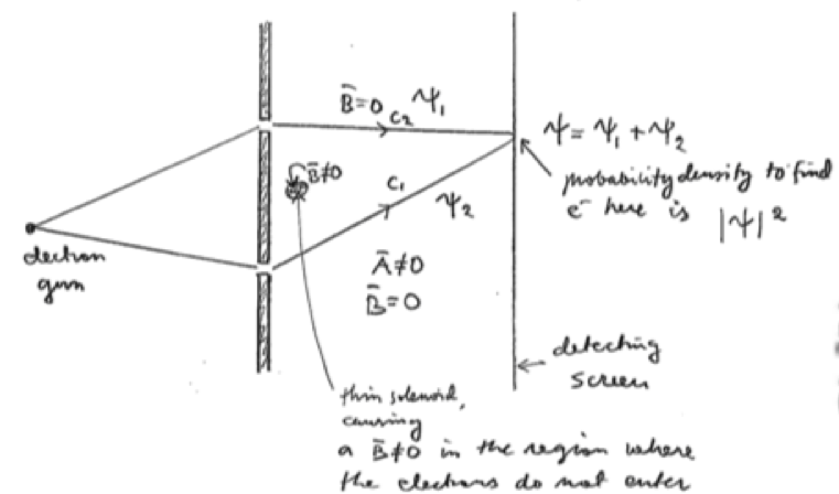
Assume there is no scalar potential, i.e., \(\varphi=0\). We wish to find out the effect of the magnetic field on the interference pattern. Within the semiclassical approximation, the propagator in the absence of the field is given by the sum of the classical paths \(C_1\) and \(C_2\). In the absence of the magnetic field, the total propagator is a sum of the form \[G_{\vec B=0}(x'',t'';x,t) = C (e^{\frac{i}{\hbar}S_{\rm cl}^1} + e^{\frac{i}{\hbar}S_{\rm cl}^2}),\] where the prefactor \(C\) describes the quantum corrections around the classical paths. Now, let us assume that in the presence of the field these quantum corrections are not affected by the field because the magnetic field vanishes along the classical paths. However, turning the field on, we get the corrections of the form \[G_{\vec B\neq 0}(x'',t'';x,t) = C (e^{\frac{i}{\hbar}S_{\rm cl}^1+\frac{iq}{\hbar}\int_{C_1} d\vec x \cdot \vec A} + e^{\frac{i}{\hbar}S_{\rm cl}^2\frac{iq}{\hbar}\int_{C_2} d\vec x \cdot \vec A}).\] The effect of the magnetic field on the phase difference between the paths is thus \[\frac{q}{\hbar}\int_{C_1} d\vec x \cdot \vec A - \frac{q}{\hbar}\int_{C_2} d\vec x \cdot \vec A=\frac{q}{\hbar} \oint d\vec x \cdot \vec A = \frac{q}{\hbar} \Phi_{12},\] where \(\Phi_{12}\) is the flux through the region spanned by the paths \(C_1\) and \(C_2\). This is thus of course nothing but the Aharonov-Bohm effect.
These are the current permissions for this document; please modify if needed. You can always modify these permissions from the manage page.