Adiabatic approximation

As a final and somewhat independent topic in the section of time-dependent phenomena, we consider an approximation method called adiabatic approximation.

Let us first take an example from classical mechanics, where we slowly move a pendulum from one position to another (say, 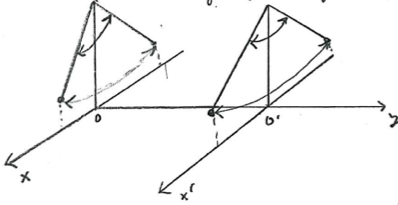$x \mapsto x'$ ): The oscillations in the two positions take place in two parallel planes, such that the state of the pendulum after movement is the same as before, but in the new coordinate system. In particular, the period and amplitude of motion remain the same.

In contrast, if we move the pendulum very suddenly, its state changes drastically.

In quantum mechanics, we can have an analogous situation for example as follows: 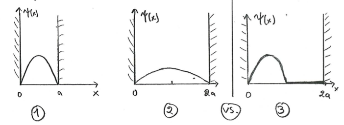Here, (1) is the starting point, and (2) and (3) correspond to an adiabatic or sudden changes to the position of the right wall. In other words, we have a quantum well of size , with infinitely high walls at x=0 and x=a . In the process we move the right wall to position x=2a and study what happens to the wave function that is initially in the ground state of the system. If we move the wall slowly [case (2)], the system remains in the ground state, and hence the wave function adiabatically adapts to the new configuration. On the other hand, in the case of a sudden change, the state of the system cannot adapt to the configuration, and immediately after the change the state is described by the same wave function as in the starting point [case (3)]. Thereafter it of course starts evolving, but now involving several excited states of the system.

Here we concentrate especially on the case (2) and try to analyze the dynamics there. Now note that we cannot apply the perturbation theory (with small H_1 ), because the changes in the system Hamiltonian are large!

In quantum mechanics, the context of the adiabatic approximation is expressed in terms of the adiabatic theorem

Suppose that $\hat H=\hat H_i$ changes gradually to $\hat H_f \neq H_i$ and that the system is originally in the th eigenstate of $\hat H_i$ . After the gradual change of $\hat H$ , the system is in the th eigenstate of $\hat H_f$ .

Proof of the adiabatic theorem

The adiabatic theorem is intuitively understandable, but let us see how we can derive it from the Schrödinger equation. For that, let us consider the eigenstates of the Hamilton operator satisfying $\hat H |\psi_k\rangle = \epsilon_k |\psi_k\rangle,$ which, for a time independent $\hat H$ are stationary states, i.e., $|\psi_k(t)\rangle = e^{-\frac{i}{\hbar} E_k t} |\psi_k\rangle.$

# timedepenergies

Now, for a time dependent $\hat H$ , we have eigenstates $\{|\psi_n(t)\rangle\}$ (different from the above set), which are not stationary, and the corresponding energy is not constant. Rather, the eigenvalue equation reads $\hat H(t) |\psi_n(t)\rangle = E_n(t) |\psi_n(t)\rangle.$ In other words, for each instant of time, $\hat H$ has different energy eigenvalues and different eigenstates. Nevertheless, since $\hat H(t)=\hat H^\dagger(t)$ , the instantaneous eigenstates form an orthonormal set: $\langle \psi_m(t)|\psi_n(t)\rangle = \delta_{mn}.$

They hence form a basis on which we can express the general state $|\psi(t)\rangle$ : $|\psi(t)\rangle = \sum_n c_n(t) e^{\overbrace{-\frac{i}{\hbar} \int_0^t dt' E_n(t')}^{i\theta_n(t)}} |\psi_n(t)\rangle,$ where the time-dependent coefficient has been written in such a way that in the time independent case c_n is also independent of time.

Now, let us substitute this state to the Schrödinger equation $i\hbar \frac{\partial}{\partial t} |\psi(t)\rangle = \hat H(t)|\psi(t)\rangle$ . We get $i\hbar \frac{d}{dt} \sum_n c_n(t) e^{i\theta_n(t)}|\psi_n(t)\rangle = \hat H(t) \sum_n c_n(t) e^{i\theta_n(t)} |\psi_n(t)\rangle = \sum_n c_n(t) e^{i\theta_n(t)} \underbrace{\hat H}_{E_n(t)} |\psi_n(t)\rangle.$ Using the chain rule to the left hand side, we get $i\hbar \sum_n e^{i\theta_n(t)}\left[\dot c_n(t)+c_n(t) \frac{d}{d t} + ic_n \underbrace{\frac{d\theta_n(t)}{dt}}_{-E_n/\hbar}\right] |\psi_n(t)\rangle = \sum_n c_n(t) e^{i\theta_n(t)} E_n(t) |\psi_n(t)\rangle.$ Here $\dot c(t)=\frac{dc(t)}{dt}$ . The last term on the left hand side cancels with the term on the right hand side. Thus we are left with $\sum_n \dot c_n(t) e^{i\theta_n(t)}|\psi_n(t)\rangle = -\sum_n c_n(t) e^{i\theta_n(t)} \frac{d}{dt} |\psi_n(t)\rangle.$

Let us multiply from the left with $e^{-i\theta_m(t)}\langle \psi_m(t)|$ . Using the orthonormality condition we hence obtain

$\boxed{\dot c_m(t) = -\sum_n c_n(t) e^{i\theta_n(t)-i\theta_m(t)} \langle \psi_m(t)|\frac{d}{dt} |\psi_n(t)\rangle.}$ What did we obtain on the right hand side? To understand it, let us take the time derivative of the equation specifying the time-dependent energies E_n(t) . We get $\frac{\partial \hat H}{\partial t} |\psi_n(t)\rangle + \hat H(t) \frac{d}{dt}|\psi_n(t)\rangle =\frac{dE_n(t)}{dt} |\psi_n(t)\rangle + E_n(t) \frac{d}{dt} |\psi_n(t)\rangle.$

Multiplying from the left by $\langle \psi_m(t)|$ and using orthonormality on the right hand side of the equation yields $\langle \psi_m(t) |\frac{\partial \hat H}{\partial t}|\psi_n(t)\rangle + \langle \psi_m(t) |\underbrace{\hat H(t)}_{E_m(t)} \frac{d}{dt} |\psi_n(t)\rangle = \frac{dE_n}{dt} \delta_{mn} + E_n(t) \langle \psi_m(t) |\frac{d}{dt} |\psi_n(t)\rangle.$ In what follows, let us consider $m\neq n$ and a non-degenerate spectrum $(E_m \neq E_n)$ . In that case the above yields $\boxed{\langle \psi_m(t)| \frac{\partial \hat H}{\partial t} |\psi_n(t)\rangle = \left[E_n(t)-E_m(t)\right]\langle \psi_m(t) |\frac{d}{dt}|\psi_n(t)\rangle.}$ Let us use this in the equation for c_m(t) . We get:

$\boxed{\frac{dc_m}{dt} = -c_m(t) \langle \psi_m(t) | \frac{d}{dt} |\psi_m(t)\rangle - \sum_{n\neq m} c_n(t) e^{i[\theta_n(t)-\theta_m(t)]} \frac{\langle \psi_m(t) |\frac{\partial \hat H}{\partial t}|\psi_n(t)\rangle}{E_n(t)-E_m(t)}},$ where $i[\theta_n(t)-\theta_m(t)]=-\frac{i}{\hbar} \int_0^t dt' [E_n(t')-E_m(t')]$ . Note that so far we haven't done any approximations: this is still an exact result.

Before we do the adiabatic approximation, notice a feature of the first term in the right hand side. We can obtain it by taking a time derivative of the normalization condition (here $|\dot \psi_m(t)\rangle = \frac{d}{dt} |\psi_m(t)\rangle$ ): $\frac{d}{dt} \langle \psi_m(t) |\psi_m(t)\rangle = \underbrace{\langle \dot \psi_m(t)|\psi_m(t)\rangle}_{=\langle \psi_m(t)|\dot \psi_m(t)\rangle^*} + \langle \psi_m(t) |\dot \psi_m(t)\rangle = \frac{d}{dt} 1 = 0.$ In other words, ${\rm Re}\left[\langle \psi_m(t) |\dot \psi_m(t)\rangle \right]=0$ or $\boxed{\langle \psi_m(t) |\dot \psi_m(t)\rangle = i\alpha(t), \quad \alpha(t) \in \mathbb{R}}$

Now we make the adiabatic approximation on the above equation: assume that the Hamiltonian is changed so slowly that the term $\frac{\partial \hat H}{\partial t}$ can be neglected. In other words, we get $\frac{d c_m}{dt} \approx -c_m(t) \langle \psi_m(t)|\dot \psi_m(t)\rangle.$ Integrating this, we get the time evolution of the state vector coefficient in adiabatic approximation: $\boxed{c_m(t) \approx c_m(0) e^{-\int_0^t dt' \langle \psi_m(t')|\frac{d}{dt'} |\psi_m(t')\rangle} \equiv c_m(0) e^{i\gamma_m(t)}}$ Here $\gamma_m=i\int_0^t dt' \langle \psi_m(t')|\dot \psi_m(t')\rangle$ is a real quantity.

It is easy to specify the adiabatic approximation: it holds when we can disregard the terms $n\neq m$ in the equation for $\frac{dc_m}{dt}$ . However, it is not equally easy to estimate its validity range in a generic setting. A general rule of thumb is that one should compare the "internal" time scales $T_i \sim \hbar/\Delta E$ , where $\Delta E$ is the relevant energy level spacing, to the "external" time scales T_e connected to the explicit time dependence in the Hamiltonian. The adiabatic approximation is valid when $T_e \gg T_i$ .

Here the relevant level spacing $\Delta E$ in a multilevel system depends on which energy level we are concentrating: when discussing a state prepared to level with index , the longest T_i is obtained by considering the energy difference to the adjacent levels m-1 or m+1 . Then it is also clear that the adiabatic approximation fails if the levels cross at some time instants.

Let the initial state now be the th eigenstate of $\hat H(t=0)$ , i.e., $c_m(0)=\delta_{mn}$ , or $|\psi(0)\rangle = |\psi_m(0)\rangle.$ In the adiabatic approximation, the coefficient evolves as $c_m(t) = \delta_{mn}e^{i\gamma_n(t)}$ so that the state vector evolves as $|\psi(t)\rangle = e^{i\gamma_n(t)} e^{i\theta_n(t)} |\psi_n(t)\rangle.$ Therefore, in the adiabatic approximation, the system remains in the th eigenstate of the time-dependent $\hat H$ ; only a couple of innocent looking phase factors are picked up.

Note that although we are not doing perturbation theory in the same sense as before, i.e., assuming $\hat H=\hat H_0+\hat V$ , where $\hat V$ is a small perturbation, we are doing perturbation theory in the sense that we assume the time dependence of $\hat H$ to be slow, so that $\frac{\partial \hat H}{\partial t} \rightarrow 0$ . Nevertheless, the overall change in the Hamiltonian over a long time period can be large!

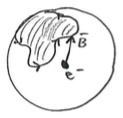
Example: electron at rest in a rotating magnetic field

Consider the following situation: 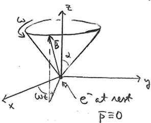The size $|\mathbf B|=B_0$ of the magnetic field is assumed to be constant, but its direction changes as in $\mathbf B(t) = B_0 \left[\sin \alpha \cos(\omega t) \hat e_x + \sin \alpha \sin(\omega t) \hat e_y + \cos \alpha \hat e_z\right].$

Let us assume that the particle is at rest $\hat p=0$ , neglect the term e^2A^2 from the vector potential, and concentrate on the spin part of the Pauli Hamiltonian. It reads $\hat H = \frac{e\hbar}{2m} \mathbf B \cdot \vec \sigma,$ where $\vec \sigma$ is a vector of Pauli spin matrices. Writing the Pauli matrices in their matrix representation yields $H(t) = \frac{\hbar \omega_1}{2} \begin{pmatrix} \cos \alpha & e^{-i\omega t} \sin \alpha \\ e^{i\omega t} \sin \alpha & -\cos \alpha \end{pmatrix},$ where $\omega_1=eB_0/m$ .

We can find the eigenspinors and eigenvalues of $\hat H(t)$ (for example using the spectral decomposition discussed earlier): $H(t)\chi_\pm(t) = E_\pm(t) \chi_\pm(t)$ with $E_\pm = \pm \frac{\hbar \omega_1}{2}, \chi_+ = \begin{pmatrix} \cos\frac{\alpha}{2} \\ e^{i\omega t} \sin\frac{\alpha}{2}\end{pmatrix}, \chi_- = \begin{pmatrix} e^{-i\omega t} \sin \frac{\alpha}{2} \\ -\cos \frac{\alpha}{2} \end{pmatrix}.$ They correspond to the spin up/down states along the instantaneous direction of $\vec B(T)$ . Note also that they satisfy $\chi_\pm^\dagger \chi_{\mp}=0$ and $\chi_{\pm}^\dagger \chi_\pm=1$ .

Let the initial state be described by $\chi(0)=\chi_+(0)=\begin{pmatrix} \cos \frac{\alpha}{2} \\ \sin\frac{\alpha}{2}\end{pmatrix}.$ This is a simple enough problem so that we can solve the Schrödinger equation exactly (in exercises). That exact solution is

# chitexact

$\begin{aligned} \chi(t) &= \begin{pmatrix} [\cos \frac{1}{2} \lambda t -i\frac{\omega_1-\omega}{\lambda} \sin \frac{1}{2} \lambda t]\cos \frac{\alpha}{2} e^{-i\omega t/2}\\ [\cos \frac{1}{2} \lambda t -i\frac{\omega_1+\omega}{\lambda} \sin \frac{1}{2} \lambda t]\sin \frac{\alpha}{2} e^{i\omega t/2}\end{pmatrix} \\ &=\left[\cos \frac{1}{2} \lambda t -i\frac{\omega_1-\omega \cos \alpha}{\lambda} \sin \frac{1}{2} \lambda t\right] e^{-i\omega t/2} \chi_+(t) + i\left[\frac{\omega}{\lambda} \sin\alpha \sin \frac{\lambda t}{2} \right] e^{i\omega t/2} \chi_-(t), \end{aligned}$ where $\lambda = \sqrt{\omega^2+\omega_1^2 -2\omega \omega_1 \cos \alpha}$ .

From this exact result, we can calculate the transition probability to the spin-down state $\chi_-(t)$ : $P_{\chi_+(0) \rightarrow \chi_-(t)}(t) =|\langle \chi_-(t)|\chi(t)\rangle |^2 = \left[\frac{\omega}{\lambda} \sin \alpha \sin \frac{\lambda t}{2}\right]^2.$ The probability of staying in the spin-up state is then $P_{\chi_+(0) \rightarrow \chi_+(t)}=1-P_{\chi_+(0)\rightarrow \chi_-(t)}$ .

The adiabatic theorem states that $P_{\chi_+(0) \rightarrow \chi_-(t)} \rightarrow 0$ when the characteristic time T_e for changes in $\hat H$ is much larger than the characteristic time T_i for changes in the wave function. Here, $T_e = \frac{2 \pi}{\omega}, \quad \text{period of rotation of } \mathbf B$ $T_i = \frac{2\pi}{\omega_1}=\frac{h}{E_+-E_-}, \quad \text{transition time between the system's states}$ The adiabatic approximation is thus valid when $T_e \gg T_i$ or $\omega \ll \omega_1$ . In this limit $\lambda = \omega_1 \sqrt{1+\left(\frac{\omega}{\omega_1}\right)^2-2\frac{\omega}{\omega_1} \cos \alpha} = \omega_1 \left[1+o\left(\frac{\omega}{\omega_1}\right)\right].$ A direct calculation then shows that $P_{\chi_+(0) \rightarrow \chi_-(t)}(t) \approx \left[\frac{\omega}{\omega_1} \sin \alpha \sin \frac{\omega_1 t}{2}\right]^2 \overset{\omega \ll \omega_1}{\rightarrow} 0$ and thus $P_{\chi_+(0) \rightarrow \chi_+(t)} \approx 1$ . The spin direction thus follows the direction of the slowly rotating magnetic field.

In the non-adiabatic regime $\omega \gg \omega_1$ , the system would rather oscillate back and forth between the spin-up and spin-down states:

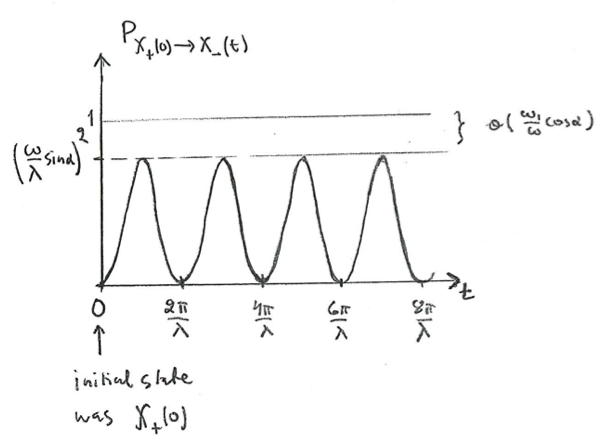
Berry's phase

Consider the following example in classical mechanics: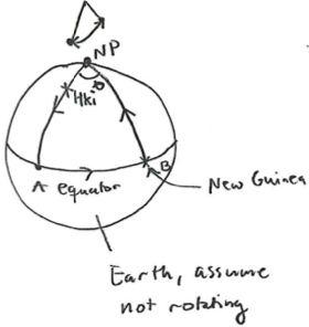

Set the pendulum to swing at the north pole into the direction of Helsinki.
Bring it down to equator adiabatically to the point A.
Bring it adiabatically to B (say, New Guinea).
Return adiabatically to the north pole.

We find that there is an angle $\theta$ between the initial and final oscillation planes. This angle does not really depend on how far south the pendulum was.

A system that does not return to its original state when transported around a closed loop is said to be nonholonomic. In quantum mechanics, we have already met such systems, for example in the case of the Aharonov-Bohm effect. Clearly, this change has something to do with the (Berry) phase of the state vector.

In the discussion of the adiabatic approximation above, we showed how, on adiabatic evolution, the system collects a phase $|\psi(t) \rangle \approx e^{i[\theta_n(t)+\gamma_n(t)]} |\psi(0)\rangle.$ Here $\theta_n = -\frac{1}{\hbar} \int_0^t E_n(t') dt'$ is called the dynamic phase and $\gamma_n = i\int_0^t dt' \langle \psi_n(t')|\dot \psi_n(t')\rangle$ is the geometric phase.

We can describe the time dependence of the Hamiltonian through some time dependent parameters. Let us denote them $R_1(t), \dots R_N(t)$ . The instantaneous eigenstates $\{|\psi_n(t)\rangle\}$ thus also depend on these parameters. Let us use the chain rule and write $\frac{d}{dt} |\psi_n[R_1(t),\dots,R_N(t)]\rangle = \left[\dot R_1(t) \frac{\partial}{\partial R_1}+\dots+ \dot R_N(t) \frac{\partial}{\partial R_N} \right]|\psi_n(R_1,\dots R_N)\rangle = \frac{d\vec R}{dt} \cdot \nabla_{\vec R} |\psi_n[\vec R(t)]\rangle,$ where $\nabla_{\vec R} = \left( \frac{\partial}{\partial R_1},\dots,\frac{\partial}{\partial R_N}\right)$ and $\vec R=\left(R_1,\dots,R_N\right).$

In this notation, the geometric phase becomes $\gamma_n(t) = i\int_0^t dt' \left\langle \psi_n[\vec R(t')]\left|\frac{d\vec R}{dt'}\cdot \nabla_{\vec R} \right|\psi_n[\vec R(t')]\right\rangle = \int_{\vec R_i=\vec R(0)}^{\vec R_f=\vec R(t)} d\vec R \cdot \underbrace{i\left\langle \psi_n[\vec R(t')]|\nabla_{\vec R} \psi_n[\vec R(t')]\right\rangle}_{\vec A_n(\vec{R})}.$ Here the quantity $\vec A_n$ is called the Berry connection. It is not unique, but depends on the chosen gauge as discussed in what follows.

If the Hamiltonian $\hat H$ returns to its original form after a time , the net geometric phase change is $\boxed{\gamma_n(T) = i\oint d\vec R \cdot \langle \psi_n(\vec R)|\nabla_{\vec R} \psi_n(\vec R)\rangle.}$ Here the integral is a line integral around a closed loop in the space of vectors $\vec R$ . This is called the Berry's phase and it was found as late as 1984 by Michael Berry.

Note that $\gamma_n(T)$ depends only on the path taken, and not how fast the path was traversed. The meaning of $\gamma_n(T)$ is obviously relevant only if this traversal was adiabatic.

In contrast, the dynamic phase $\theta_n(T)$ depends on . For instance, take a beam of particles, in a state $\psi$ , split it into two halves, and make one half go through an adiabatically changing potential and the other half not. Combining the beams into one beam again corresponds to $\psi=\frac{1}{2}\psi_0 + \frac{1}{2} \psi_0 e^{i\Gamma}.$ Hence the probability amplitude is $|\psi|^2 = |\psi_0|^2 \cos^2 \frac{\Gamma}{2} \neq |\psi_0|^2.$ In other words, such relative phases can be measured in interference patterns.

Gauge transformations, Berry connection and Berry curvature

Let us consider a gauge transformation, transforming the chosen basis by a phase factor that depends on $\vec R$ : $|\psi_n'[\vec R(t)]\rangle = e^{-i\beta(\vec R)}|\psi_n[\vec R(t)]\rangle.$ As a result, the Berry connection changes: $\vec A_n'(\vec{R})=\vec A_n(\vec{R}) + \nabla_{\vec R} \beta(\vec R)$ . In other words, it is not gauge invariant and hence not physically observable.

Let us take a derivative in direction $\mu$ of the $\nu$ component of the Berry connection and subtract the derivative in direction $\nu$ of the $\mu$ component. We get the Berry curvature $\Omega_{n,\mu\nu}(\vec R) \equiv \frac{\partial A_{n\nu}(\vec R)}{\partial R^\mu} - \frac{\partial A_{n\mu}(\vec R)}{\partial R^\nu}$ It is an anti-symmetric second-rank tensor.

Let us next consider three-dimensional parameter space. In this case, the Berry curvature can be defined via $\vec \Omega_n=\nabla_{\vec R} \times \vec A_n(\vec R)$ . You may see a formal connection to the magnetic field and the vector potential. The two definitions can be put together by noting that the Berry curvature vector $\vec \Omega_n$ is connected to the antisymmetric Berry curvature tensor by $\Omega_{n,\mu\nu}=\epsilon_{\mu\nu\xi} \mathbf \Omega_{n,\xi}$ with the Levi-Civita symbol $\epsilon_{\mu\nu\xi}$ .

Moreover, since gradient fields produce no curl, the Berry curvature is gauge invariant: $\vec \Omega_n' \equiv \nabla_{\vec R} \times \vec A_n'(\vec R) = \nabla_{\vec R} \times [\vec A_n(\vec R)+\nabla_{\vec R} \beta(\vec R)]=\nabla_{\vec R} \times \vec A_n(\vec R) = \vec \Omega_n.$

Now for any closed path $\cal C$ enclosing a surface $\cal S$ we can use the Stokes theorem so that the Berry phase can be expressed as $\gamma_n(T)=\int_{\cal C} d\vec R \cdot \vec A_n(\vec R) = \int_{\cal S} d\vec S \cdot \mathbf \Omega_{n}$ The gauge invariance of the Berry curvature then implies that the Berry phase is independent of the chosen gauge.

On the other hand, if the surface ${\cal S}$ is a closed manifold (sphere of a ball, torus, etc.), according to the Gauss-Bonnet theorem the Berry phase has to be an integer multiple of $2\pi$ . It therefore does not directly affect physical observables, but it has a role in characterizing quantization effects in topological matter.

Example of the Berry phase, spin $\frac{1}{2}$ in a rotating magnetic field

Let us again consider the example of the spin $\frac{1}{2}$ particle in a rotating magnetic field. From the exact solution, we see that in the adiabatic regime $\omega \ll \omega_1$ we have $\lambda \approx \omega_1 \left(1-\frac{\omega}{\omega_1} \cos \alpha\right)=\omega_1-\omega \cos \alpha$ and $\chi(t) \approx e^{-i\omega_1 t/2} e^{i\omega \cos(\alpha) t/2}e^{-i\omega t/2} \chi_+(t) +i\underbrace{\left[\frac{\omega}{\omega_1} \sin \alpha \sin \frac{\omega_1 t}{2}\right]}_{\rightarrow 0 \text{ for } \omega \ll \omega_1} e^{i\omega t/2}\chi_-(t).$

The dynamic phase is now ( $E_\pm = \pm \hbar\omega_1 /2$ ) $\theta_+(t) = -\frac{1}{\hbar} \int_0^t dt' E_+(t') = -\frac{\omega_1 t}{2}.$

On the other hand, the geometric phase is $\begin{aligned} \gamma_+(t) &= i\int_0^t dt' \chi_+^\dagger(t') \dot \chi_+(t') = i \int_0^t dt' \begin{pmatrix} \cos \frac{\alpha}{2} & e^{-i\omega t'} \sin \frac{\alpha}{2} \end{pmatrix} \begin{pmatrix} 0 \\ i\omega e^{i\omega t'} \sin \frac{\alpha}{2} \end{pmatrix}\\ &=i\int_0^t dt' i\omega \sin^2 \frac{\alpha}{2} = \frac{\omega t}{2} (\cos \alpha-1). \end{aligned}$

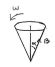
The Berry phase requires a complete cycle, i.e., $T=2\pi/\omega$ . There, $\gamma_+(T)=\pi (\cos \alpha-1) = -\frac{1}{2} \int_0^{2\pi} d\varphi \int_0^\alpha d\alpha \sin \alpha = -\frac{1}{2} \int_{\Omega_\alpha} d\Omega,$ where $\Omega_\alpha$ is the solid angle swept by $\mathbf B$ .

This example generalizes to the case where the tip of the $\mathbf B$ vector sweeps out an arbitrary closed curve on the surface of a sphere of radius r=B_0 : Also in this case $\gamma_+(T)=-\frac{1}{2} \int d\Omega = -\frac{1}{2} \Omega$ .

Moreover, for a particle of spin , the above result generalizes to $\gamma_+(T)=-S\Omega$ .

Aharonov-Bohm effect and Berry's phase

During the previous week we encountered the Aharonov-Bohm effect where the relative phases between different particle paths can be controlled by magnetic fluxes. Here we show how the effect is actually a manifestation of the Berry's phase.

Case 1:

Particle constrained to move in a circle of radius around an infinitely long solenoid 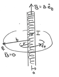Here: =particle's charge, =current in the solenoid, =solenoid radius, $\vec B$ =constant magnetic field inside the solenoid, i.e., for r<a , whereas $\vec B=0$ outside the solenoid, r> a .

The magnetic flux through the ring at r>a is $\begin{aligned} \Phi &= \pi a^2 B = \int_r d\vec S \cdot \vec B =\int d\vec S \cdot (\nabla \times \vec A) \overset{\rm Stokes}{=}\oint d\vec r \cdot \vec A(r) =\int_0^{2\pi} d\varphi r \hat e_\varphi \cdot \vec A(r) \end{aligned}$ This works with $\vec A(r) = \frac{A_0}{r} \hat e_\varphi$ and $A_0=\frac{\Phi}{2\pi}$ , at any point with . Namely, this choice of the vector potential satisfies $\vec B = \nabla \times \vec A(r)=0$ and $\nabla \cdot \vec A(r)=0$ (Coulomb gauge).

Let us now incorporate this to the Hamiltonian for a spinless particle (spin is not important for the regular Aharonov-Bohm effect). In other words, $\begin{aligned} \hat H = \frac{1}{2m}\left(\hat {\mathbf p}-q \mathbf A\right)^2 \overset{\nabla \cdot \mathbf A=0}{=} \frac{1}{2m} \left[-\hbar^2 \nabla^2 + q^2 A^2 +2i\hbar q \mathbf A \cdot \nabla \right]. \end{aligned}$

Now, since the particle is bound to move at r=b , we can simplify, in cylindrical coordinates $\begin{aligned} \nabla = \hat e_r \underbrace{\frac{\partial}{\partial r}}_{=0} + \hat e_\varphi \frac{1}{r} \frac{\partial}{\partial \varphi} + \hat e_z \underbrace{\frac{\partial}{\partial z}}_{=0} \overset{r=b}{=} \hat e_\varphi \frac{1}{b} \frac{\partial}{\partial \varphi}. \end{aligned}$

Substituting to the Schrödinger equation, we get $\begin{aligned} \frac{1}{2m}\left[-\frac{\hbar^2}{b^2} \frac{\partial^2}{\partial \varphi^2} + \left(\frac{q\Phi}{2\pi b}\right)^2 +i\frac{\hbar q \Phi}{\pi b^2} \frac{\partial}{\partial \varphi} \right]\psi(\varphi) = E \psi(\varphi) \end{aligned}$ or $\begin{aligned} \psi''(\varphi)-2i\beta \psi'(\varphi)+\epsilon \psi(\varphi)=0, \end{aligned}$ where $\beta=\frac{q\Phi}{2\pi \hbar}$ and $\epsilon = \frac{2mb^2 E}{\hbar^2}-\beta^2$ are constants characterizing the flux and the energy.

The solutions are of the form $\psi(\varphi)=A e^{i\varphi \lambda}$ with $\lambda = \beta \pm \sqrt{\beta^2+\epsilon} = \beta \pm \frac{b}{\hbar} \sqrt{2mE}.$ They also have to be consistent, i.e., satisfy $\psi(\varphi+2\pi)=\psi(\varphi)$ . This means that $\lambda=n \in {\mathbb Z}$ . In other words, we get discrete energies $E_n =\frac{\hbar^2}{2mb^2} \left(n-\frac{q\Phi}{2\pi \hbar}\right)^2, \quad n=0, \pm 1, \pm 2, \dots$ The particle energies thus depend on the flux through the solenoid in a region where those particles do not enter at all! This implies persistent currents in the ring (see for example this recent measurement), but that topic is outside the context of this course.

Case 2

Let the particle move more freely now, but in the region where $\vec B=0$ . In other words, $\nabla \times \vec A = 0$ , but still $\vec A\neq 0$ . Let $\vec A$ be static for simplicity.

The Schrödinger equation reads $\begin{aligned} \left[\frac{1}{2m}\left(\frac{\hbar}{i} \nabla - q\vec A\right)^2+V\right]\psi=i\hbar \frac{\partial \psi}{\partial t}. \end{aligned}$

Let us now use the following trick, similar to when discussing the gauge invariance. We write $\begin{aligned} \psi(t,\vec r) = e^{ig(\vec r)} \psi'(t,\vec r), \quad g(\vec r) = \frac{q}{\hbar} \int_O^{\vec r} d\vec r' \cdot \vec A(\vec r'), \end{aligned}$ where the integral is calculated along an arbitrary path from point to point $\vec r$ , but such that along the path $\vec B=0$ .

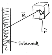
Now $\nabla g(\vec r)=\frac{q}{\hbar} \vec A$ so that $\psi'$ satisfies an equation not containing $\vec A$ , $\begin{aligned} \left[\frac{\hbar^2}{2m}\nabla^2+V\right]\psi'=i\hbar \frac{\partial \psi'}{\partial t}. \end{aligned}$ Aharonov and Bohm proposed to carry out the following experiment: 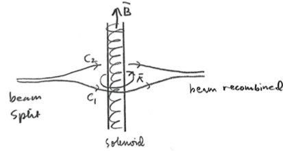For such an arrangement, the phase difference of the recombining beams is $g_1-g_2=\frac{q}{\hbar} \int_{C1-C2} \vec{A} \cdot d\vec r = \frac{q}{\hbar}\Phi.$ Here the path C_1-C_2 means traversing along path C_1 forward first, and then backwards in the path C_2 (i.e., implying a negative sign for this contribution). As a result, the path goes around the whole solenoid, and by Stokes theorem the phase difference can again be associated to the total flux through the solenoid.

In practice, Aharonov-Bohm effect is measured in specially prepared conducting rings. For example, the effect was measured in graphene as shown in this paper.

Connection between the Aharonov-Bohm effect and Berry's phase

Assume a particle confined inside a box by a potential $V(\vec r-\vec R)$ , and carry this box with the particle around the solenoid (i.e., $\vec R=\vec R(t)$ ):

The instantaneous energy eigenstates are now obtained from $\begin{aligned} \left\{\frac{1}{2m}\left[-i\hbar \nabla - q \vec A(\vec r)\right]^2 +V(\vec r-\vec R)\right\}\psi_n(\vec r) = E_n \psi_n(\vec r). \end{aligned}$

Let us again make the gauge transformation, but choosing the origin to the center of the box: $\begin{aligned} \psi_n = e^{ig(\vec r,\vec R)} \psi_n'(\vec r-\vec R), \quad g(\vec r,\vec R) = \frac{q}{\hbar} \int_{\vec R}^{\vec r} d \vec r' \cdot \vec A(\vec r'). \end{aligned}$ As above, it is straightforward to show that $\psi'$ satisfies an equation without $\vec A$ : $\begin{aligned} \left(-\frac{\hbar^2}{2m} \nabla^2 + V(\vec r-\vec R)\right)\psi_n' = E_n \psi_n'. \end{aligned}$

Remember, to get the Berry's phase we want to evaluate $\langle \psi_n |\nabla_{\vec R} \psi_n \rangle$ . For that, let us first calculate $\nabla_{\vec R} \psi_n(\vec r-\vec R) = \nabla_{\vec R} e^{ig(\vec r,\vec R)} \psi_n'(\vec r-\vec R)= -i\frac{q}{\hbar} \vec A(\vec R) e^{ig} \psi_n'(\vec r-\vec R) + e^{ig} \nabla_{\vec R} \psi_n'(\vec r-\vec R).$ Then $\begin{aligned} \langle \psi_n |\nabla_{\vec R} \psi_n \rangle &= \int d^3 \vec r e^{-ig} (\psi_n')^*(\vec r-\vec R)e^{ig} \left[-i\frac{q}{\hbar} \vec A(\vec R)\psi_n'(\vec r-\vec R)+\nabla_{\vec R} \psi_n'(\vec r-\vec R)\right]\\ &=-i\frac{q}{\hbar} \vec A(\vec R)+\underbrace{\int d^3\vec r (\psi_n')^*(\vec r-\vec R)\underbrace{\nabla_{\vec R} \psi_n'(\vec r-\vec R)}_{=-\nabla_{\vec r} \psi_n'(\vec r-\vec R)}}_{=0 \text{ (in a box)}} = -i\frac{q}{\hbar} \vec A(\vec R). \end{aligned}$

To get the Berry phase, we need to make a closed line integral over the path $\vec R(t)$ . Therefore, we now assume that the box moves around the solenoid. In this case $\begin{aligned} \gamma_n(T) = \frac{q}{\hbar} \oint d\vec R \cdot \vec A(\vec R) \overset{\rm Stokes}{=} \frac{q}{\hbar} \int d\vec S \cdot \left[\underbrace{\nabla \times \vec A(\vec R)}_{=\vec B(\vec R)}\right] = \frac{q}{\hbar} \Phi, \end{aligned}$ where $\Phi$ is the magnetic flux through the region spanned by the circular path $\vec R$ , i.e., the one through the center of the solenoid.

In other words, the Aharonov-Bohm effect is a special case of the Berry phase.