Learning goals for this week (check afterwards that you understand these concepts)
- Understanding the concept of the scattering experiments
- QM formulation of the scattering experiment
- Cross section, differential cross section
- Integral equation for scattering and the Green's function of the scattering problem
- Complex integration; residue theorem; transforming an integral over a real axis to a closed complex line integral
- Solving for the Green's function via complex integration
- Born series solution of the integral equation; Born approximation
Basic concept: cross section
The structure of matter is probed by doing
Spectroscopy: observe transitions between the different bound states at the system (atoms, molecules,
 ) - analyzed with the methods of the time-dependent perturbation theory, often with harmonic perturbations.
Scattering experiments: analyze the final states and deduce the properties of target and/or beam particles (for example the structure and properties of nuclei and elementary particles, or nature of electron transport inside solids)
A typical scattering experiment (with a fixed target) could look like this: 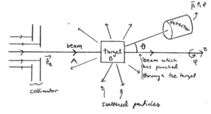

It thus consists of two parts:
beam:
consists of particles A (electrons, positrons, protons, neutrons, photons, phonons,
)is nearly monoenergetic and well collimated:
 (allows considering a given input energy/momentum)
target: (fixed target
 macroscopic sample)
consists often of a large number of particles B (e.g., H-gas in a container, stack of lead plates, etc.)
or an impurity potential in a solid (dislocations, vacancies, and other irregularities of the ion lattice)
One can generally separate the scattering to two categories:
Elastic scattering:
 Same particles in the initial and final states, i.e., total kinetic energy is conserved
Inelastic scattering: final state particles
 initial state particles, or the structure of A,B can change.
For example: 
 could be for example
 : elastic scattering
 : excitation of
 : ionization of
  : annihilation
") : positronium formation
: positronium formation
(ii)-(v) are inelastic
The "final state" particles are taken to a detector, which can then measure for example the magnitude of their momentum (or their kinetic energy)  as a function of the angles
  ,
,  . In addition, the detector can be sensitive to the polarization, spin, or some other internal property of the output beam.
A key quantity in scattering experiments is the cross section for scattering  = number of these scattering events per unit time, per one target particle B, divided by the flux of incoming beam particles A
Let's illustrate it here:
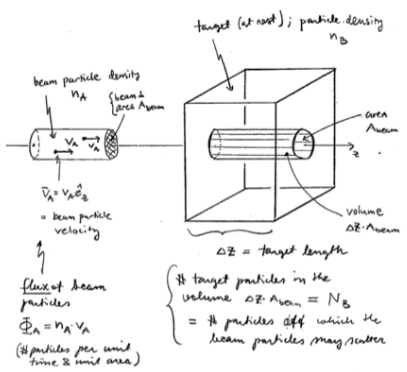
Let us assume that the detector observes the number  of scattering events in a unit time. Obviously, the more flux
  and the larger
  , the larger must be:
We can therefore define the scattering cross section as 
It depends on the scattering process considered, i.e., on the probability of scattering, i.e., on the strength and range of the interaction and the beam energy
Here  is an effective "cross section" which the beam particles see. It is also related to the probability for the scattering to happen. These have the physical units:
 \\
[N_B] &= 1\\
[\sigma] &= {\rm length}^2.\end{aligned}")
Units used in nuclear and particle physics:  1 b = 1 barn = 10
 m
m = 100 fm.
Often, it is not easy to detect the particles scattered in all possible directions, or there is extra information in the precise angle to which the scattering takes place. Therefore, one often also considers the differential cross section }{\Phi_A N_B},") where
where  d\Omega") is the number of particles per unit time, scattered into the infinitesimal solid angle
is the number of particles per unit time, scattered into the infinitesimal solid angle  :
: 
For example experimental figures on scattering cross sections in particle physics, see for example K. Nakamura, et al., Review of Particle Physics, J. Phys. G: Nucl. Part. Phys. 37, 075021 (2010).
You can get more information on particle physics measurements in the course FYSS4300 Particle Physics.
In this chapter,
We formulate the general 3d scattering problem, where the wave function far away from the scattering region satisfies
=\underbrace{A e^{ikz}}_{\rm incoming} + \underbrace{f(\theta,\varphi) \frac{e^{ikr}}{r}}_{\rm outgoing}.") The rest of the chapter deals with methods aiming to solve
The rest of the chapter deals with methods aiming to solve ") .
.We use the Green's function technique to transform the Schrödinger equation to an integral equation. This is then solved with the Born approximation. It is especially useful for weak potentials, where the deviation of the particle's initial trajectory is small.
Another approach is the partial wave analysis, where the
dependence is expanded in terms of the spherical harmonics. This method is useful especially for low-energy particles (compared to the potential strength), since for that case ") is a weak function of
is a weak function of 
Alternatively to the lecture notes, you may also follow Ch. 11 in Griffiths' book.
Formulation of the 3d scattering problem: boundary conditions of the wave function, cross section, optical theorem
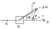
We consider here the elastic scattering of two spinless, nonrelativistic particles. In laboratory frame, the incoming particles have a certain momentum and the target is at rest (sometimes referred to as the target rest frame). In the center-of-momentum (CMS) frame, the total momentum of an incoming particle and a target particle is zero: 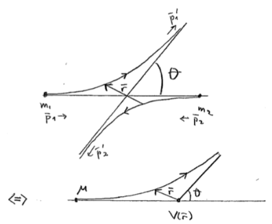
In the CMS frame the total momentum of the system vanishes, and hence  , the relevant energy is the relative kinetic energy between the particles, and the relevant position is the relative position,
  . This is equivalent to a scattering of a particle of a reduced mass
 ") of a potential
of a potential ") .
.
In order to be able to calculate the cross section, we must assume a finite-range, localized (and often spherically symmetric) potential ") ;
;  \xrightarrow{r\rightarrow \infty} 0") :
: 
We proceed analogously to what was done in QM I in the case of a 1D problem (Griffiths, Ch. II). Instead of using calculationally much more difficult wave packets and their time evolution to describe particles and their motion, we assume a stationary situation, i.e., that the beam has been "turned on" already for a while and that we thus have a steady flux of incoming and scattered particles. This "turning on" is described in more detail in the chapter on time-dependent phenomena. We thus consider the scattering problem within the following framework:  That is, at
  , the particles behave as free,
  \rightarrow 0") .
.
Let us first specify the incoming plane wave in the 3d case, far away from the scattering center  . The stationary Schrödinger equation reads in the position representation
 = E \Psi({\mathbf r})") This is solved with the plane wave solution (prefactor comes from the properties of Fourier transformation)
This is solved with the plane wave solution (prefactor comes from the properties of Fourier transformation) =\frac{1}{(2\pi)^{3/2}} e^{i {\mathbf k}\cdot {\mathbf r}}, \quad k^2=\frac{2\mu E}{\hbar^2}}") This is hence the form of the wave function for the beam of particles far away from the scattering center.
This is hence the form of the wave function for the beam of particles far away from the scattering center.
For a radially symmetric potential, we can make the separating Ansatz =R(r) Y_{lm}(\Omega)") (see Griffiths, Ch. IV). There,
(see Griffiths, Ch. IV). There, ") satisfies the radial Schrödinger equation
satisfies the radial Schrödinger equation  + \underbrace{\frac{\hbar^2 l (l+1)}{2\mu r^2}}_{\text{This one remains}} + \underbrace{V(r)}_{\rightarrow 0 \text{ as } r\rightarrow \infty}\right] R(r) = E R(r),") i.e., we assume
i.e., we assume ") to decay faster than the centrifugal term
to decay faster than the centrifugal term /r^2") at large
at large  . In other words,
 +2r R'(r)+[(kr)^2-l(l+1)]R(r) = 0}")
The general solution to this can be specified in terms of spherical Bessel (") ) and Neumann
) and Neumann )") functions:
functions: =A j_l(kr) + B n_l(kr)") For large arguments, they have the asymptotic behavior
For large arguments, they have the asymptotic behavior  &\xrightarrow{x \gg l(l+1)/2} \frac{1}{x} \sin(x-l \pi/2) = \frac{1}{x} \frac{1}{2i} \left(e^{i(x-l \pi/2)} - e^{-i(x-l \pi/2)}\right)\\
n_l(x) &\xrightarrow{x \gg l(l+1)/2} -\frac{1}{x} \cos(x-l \pi/2) = -\frac{1}{x} \frac{1}{2} \left(e^{i(x-l \pi/2)} + e^{-i(x-l \pi/2)}\right)\end{aligned}")
For a large , the solution to the radial equation can hence be written in terms of plane waves:  \xrightarrow{kr \rightarrow \infty} \frac{1}{2kr}\left[\left(\frac{A}{i}-B\right) e^{-il \pi/2} \underbrace{e^{ikr}}_{\text{\parbox{1cm}{outgoing wave?}}} + \left(-\frac{A}{i}-B\right) e^{il \pi/2} \underbrace{e^{-ikr}}_{\text{\parbox{1cm}{incoming wave?}}}\right]}.")
Identification in terms of incoming and outgoing waves can be done by considering the probability flux, or probability current density  \nabla \Psi({\mathbf r}) - (\nabla \Psi^*({\mathbf r})) \Psi({\mathbf r})\right]
=\frac{\hbar}{\mu} {\rm Im}[\Psi^*({\mathbf r}) \nabla \Psi({\mathbf r})]}.") This can be derived from the general continuity equation defining a relation between the probability density and probability current density.
This can be derived from the general continuity equation defining a relation between the probability density and probability current density.
Generally in physics current densities can be defined in terms of the continuity equation relating the current density  and the corresponding density
  (say, charge density, particle density, probability density,)
  The continuity equation basically states that spatial variations in the current are accompanied by changes (in time) of the density, or in other words, time-dependent changes in density result into spatial dependence of the current.
Now consider the probability density in quantum mechanics, i.e., = |\Psi({\mathbf r})|^2,") Its time derivative satisfies
Its time derivative satisfies \\
&=\frac{i}{\hbar} (\Psi H^* \Psi^*-\Psi^* H \Psi)\end{aligned}") Now use the position representation of the Hamiltonian,
Now use the position representation of the Hamiltonian, +V({\mathbf r})") . The potential commutes with
. The potential commutes with ") and hence can be dropped. Moreover, we can use
and hence can be dropped. Moreover, we can use .")
As a result, we get  \equiv -\nabla \cdot {\mathbf j}.") We hence found an expression for the current density in terms of the wave function
We hence found an expression for the current density in terms of the wave function  = \frac{\hbar}{m} {\rm Im}(\Psi^* \nabla \Psi).}")
For the plane wave solution describing the incoming wave, ^{-3/2} e^{i{\mathbf k}\cdot {\mathbf r}}") , we get
, we get ^3} \frac{\hbar {\mathbf k}}{\mu}}
\end{align*}") In defining the cross section, we need the amount (per unit time) of scattered particles moving through a sphere surface at :
In defining the cross section, we need the amount (per unit time) of scattered particles moving through a sphere surface at :  Recall the spherical-coordinates representation of gradient:
 ") so that
so that  \nabla \Psi({\mathbf r})]_r = \frac{\hbar}{\mu} {\rm Im}[R^*(r) R'(r) Y_{lm}^*(\Omega) Y_{lm}(\Omega)].")
1=jin
Comparing to the generic solution to the radial equation we hence want to see what happens with =C e^{\pm ikr}/r") . Direct calculation gives
. Direct calculation gives  \underbrace{\int d\Omega Y_{\rm lm}^*(\Omega) Y_{\rm lm}(\Omega)}_{=1}\right] = \pm |C|^2 \frac{\hbar k}{\mu}.") The total particle flux is thus independent of the radial coordinate , which is desired because there are no sources or sinks of particles. Now we can identify what the signs mean:
The total particle flux is thus independent of the radial coordinate , which is desired because there are no sources or sinks of particles. Now we can identify what the signs mean:
"+" outgoing spherical wave
"-" incoming spherical wave
Moreover, we find that the proper asymptotic behavior of an outgoing spherical wave is  .
.
Now we are in position of defining the quantum scattering problem:
Quantum scattering problem
With a potential decaying faster than  , find the solutions of the spherical Schrödinger equation
 + V({\mathbf r}) \Psi({\mathbf r}) = E \Psi({\mathbf r})") or
or  \Psi({\mathbf r}) = U({\mathbf r}) \Psi({\mathbf r}), \quad \text{ where } U({\mathbf r}) \equiv \frac{2\mu}{\hbar^2} V({\mathbf r})}") fulfilling the boundary condition
fulfilling the boundary condition
 \xrightarrow{r\rightarrow \infty} \frac{1}{(2\pi)^{3/2}} \left[\underbrace{e^{i{\mathbf k}\cdot {\mathbf r}}}_{\text{\parbox{1.5cm}{incoming particles}}} + \underbrace{\frac{e^{ikr}}{r} f_k(\theta,\varphi)}_{\text{\parbox{3cm}{spherical outgoing wave $\cong$ scattered particles}}}\right]}") Here
Here =\text{ scattering amplitude}.}")
For the wave function modulus squared  to integrate (over all space) to probabilities (dimensionless number), the units of the wave function have to be
  . This unit is thus ''hidden'' in the normalization constant. The square bracket is dimensionless, so the scattering amplitude must have units
  .
.
We have two remaining problems: What is ") if is known? What is the relation between and the scattering cross section ?
if is known? What is the relation between and the scattering cross section ?
Note that is a generalization of the transmission and reflection probability amplitudes from the one-dimensional scattering problem.
To answer the second question, let us check the particle fluxes for our Ansatz asymptotic wave function. The total flux is  \nabla \Psi({\mathbf r})] = {\mathbf j}_{\rm in}+{\mathbf j}_{\rm scatt} + {\mathbf j}_{\rm int}\\
\overset{r \rightarrow \infty}{=}& \frac{\hbar}{\mu} {\rm Im}[\underbrace{\Psi_{\rm in}^*({\mathbf r}) \nabla \Psi_{\rm in}({\mathbf r})}_{\propto {\mathbf j}_{\rm in}}+\underbrace{\Psi_{\rm scatt}^*({\mathbf r}) \nabla \Psi_{\rm scatt}({\mathbf r})}_{\propto {\mathbf j}_{\rm scatt}} \\&+\underbrace{\Psi_{\rm in}^*({\mathbf r}) \nabla \Psi_{\rm scatt}({\mathbf r})+ \Psi_{\rm scatt}^*({\mathbf r}) \nabla \Psi_{\rm in}({\mathbf r})}_{\propto {\mathbf j}_{\rm int}}].\end{aligned}")
Therefore, we find that the total current consists of three parts. The first of these is nothing but the flux of incoming particles, denoted above. To understand the second, let us consider the number of particles scattered into a solid angle in a unit time per target particle  d\Omega \overset{r \rightarrow \infty}{=} {\mathbf dS} \cdot {\mathbf j}_{\rm scatt} = r^2 d\Omega (j_{\rm scatt})_r.") Here
Here  \nabla \Psi_{\rm scatt}({\mathbf r})]=\frac{1}{(2\pi)^3} \frac{\hbar}{\mu} {\rm Im}\left[\frac{e^{-ikr}}{r} f_k^*(\Omega) \nabla\left(\frac{e^{ikr}}{r}f_k(\Omega)\right)\right].") In other words,
In other words, _r = \frac{1}{(2\pi)^3} |f_k(\Omega)|^2 \frac{\hbar k}{\mu} \frac{1}{r^2}.") and therefore
and therefore _r = \frac{1}{(2\pi)^3} |f_k(\theta,\varphi)|^2 \frac{\hbar k}{\mu} d\Omega.")
Using  from Eq. (1) we can hence define the cross section,
  d\Omega}{N_B}") yielding
yielding |^2} \quad \text{elastic cross section}") and where
and where |^2} \quad \text{differential cross section.}") As the scattering amplitude has units , it makes sense that
As the scattering amplitude has units , it makes sense that  has units of the (differential) cross section, i.e.,
  .
.
We have thus answered the second question above: finding the (absolute value of the) scattering amplitude amounts to calculating the differential cross section. In retrospect it is quite clear that the two quantities must contain the same information, because they are the only ingredients left open after specifying the scattering setup!
1=jin
Before proceeding to the methods to calculate , let us fix one loose end: what happens to the interference current term  ? It is given by
 ^3} {\rm Im}[e^{-i{\mathbf k}\cdot {\mathbf r}} \nabla(\frac{e^{ikr}}{r}f_k(\Omega))+\frac{e^{-ikr}}{r} f_k^*(\Omega) \nabla e^{i{\mathbf k}\cdot {\mathbf r}}].\end{aligned}") Its radial component becomes
Its radial component becomes _r=\frac{\hbar}{\mu} \frac{1}{(2\pi)^3} {\rm Im}\left[e^{-ikr\cos(\theta)} f_k(\Omega) \underbrace{\partial_r \frac{e^{ikr}}{r}}_{\frac{e^{ikr}}{r}(ik-1/r)} + \frac{e^{-ikr}}{r} f_k^*(\Omega) \underbrace{\partial_r e^{ikr\cos(\theta)}}_{ik\cos(\theta) e^{ikr\cos(\theta)}}\right],") where we defined the spherical angle by the relation
where we defined the spherical angle by the relation ") .
.
Proceeding, we get _r \overset{r\rightarrow \infty}{=} \frac{\hbar}{\mu} \frac{1}{(2\pi)^3} {\rm Im}\left[\frac{ik}{r} (f_k(\theta,\varphi) e^{ikr(1-\cos(\theta))} + \text{complex conjugate}) + o\left(\frac{1}{r^2}\right)\right].") Now, when
Now, when  \neq 0") ,
, }") oscillates very rapidly when .
oscillates very rapidly when .
So far we have assumed that the incoming beam is entirely monoenergetic, i.e., contains only a single wave vector. This certainty of momentum would correspond to a wave packet with an infinite spread in space. In reality, the beam is never monoenergetic, but contains some spread  in the wave number. This spread is not very relevant for the incoming and outgoing currents, but it matters in the case of the very rapidly oscillating interference current. Therefore, let us average over this spread with some weight function
 ") . That means that when we compute the flux across a spherical surface at , we should replace
. That means that when we compute the flux across a spherical surface at , we should replace  \mapsto r^2 \int d\Omega \int dk g(k) j_r(r,\theta,\varphi;k),") where is a smooth function of
where is a smooth function of  , with a spread
  around some maximal value of . Generally is set by the experiment in question.
This means that now we have integrals of the type  f_k}_{\text{smooth in k}} \exp(ikr\underbrace{(1-\cos \theta)}_{\neq 0}) = 0.") Generally, these sort of arguments can be related to the Riemann-Lebesgue lemma.
Generally, these sort of arguments can be related to the Riemann-Lebesgue lemma.
Therefore, the oscillating terms appearing at  vanish. Let us include only the integration near
  :
: ^3} r^2 \int_0^{2\pi} d\varphi \int_{1-\cos \delta\theta}^1 d(\cos\theta) {\rm Im}[\frac{ik}{r}(f_k(0) e^{ikr(1-\cos(\theta))} + \text{complex conj.}) + o(1/r^2)]\\
&=\frac{\hbar}{\mu} \frac{1}{(2\pi)^3} 2\pi r^2 {\rm Im}[\frac{ik}{r}f_k(0)\frac{1}{-ikr} e^{-ikr(1-\cos(\theta))}|_{1-\cos \delta\theta}^1 + c.c. + o(1/r^2)]\\
&=\frac{\hbar}{\mu} \frac{1}{(2\pi)^3} 2\pi r^2 {\rm Im}[\frac{i}{r^2} (if_k(0) \{1-e^{ikr \cos(\delta \theta)}\} + c.c.) + o(1/r^2)]\\
&=-\frac{\hbar}{\mu} \frac{1}{(2\pi)^3} 2\pi {\rm Im}[f_k(0) -f_k^*(0) + o(1/r^2)]\\
&=-\frac{\hbar}{\mu} \frac{1}{(2\pi)^3} 4 \pi {\rm Im}[f_k(0)] + o(1/r^2).\end{aligned}")
So what is the consequence of this lengthy calculation? Recall the continuity equation +\nabla \cdot {\mathbf j}= 0,") where is the (probability or particle) density. In the stationary case the first term vanishes, and the continuity equation is a statement of probability flux conservation. In other words,
where is the (probability or particle) density. In the stationary case the first term vanishes, and the continuity equation is a statement of probability flux conservation. In other words, _r+(j_{\rm scatt})_r+(j_{\rm int})_r].\end{aligned}")
The incoming current satisfies _r=(2\pi)^{-3} \hbar k/\mu (\hat e_z)_r=(2\pi)^{-3} \hbar k/\mu \cos(\theta)") and therefore
and therefore _r \propto \int_{-1}^1 d(\cos(\theta)) \cos(\theta) =0.") In other words, the incoming current brings in (say, from the left) equally much current as they take out (say, to the right). On the other hand, the scattered total current is
In other words, the incoming current brings in (say, from the left) equally much current as they take out (say, to the right). On the other hand, the scattered total current is _r = \frac{1}{(2\pi)^3} \frac{\hbar k}{\mu} \underbrace{\int d\Omega |f_k(\Omega)|^2}_{\sigma_{\rm tot}}.")
Combining the continuity equation and our result for the interference current, we get the optical theorem ]}") According to the optical theorem, which we have now derived, the total cross section is related to the imaginary part of the forward scattering amplitude. Physically, this means that behind the target, at
According to the optical theorem, which we have now derived, the total cross section is related to the imaginary part of the forward scattering amplitude. Physically, this means that behind the target, at  , the incoming wave and the scattered wave interfere destructively, so that the intensity of the beam which has passed the target decreases by an amount which is proportional to the total cross section.
Integral equation for (potential) scattering
After having specified the scattering problem, we should try to solve it at least in some particular cases. In other words, we wish to solve the 3d differential equation
 \Psi({\mathbf r})= U({\mathbf r}) \Psi({\mathbf r})") with the asymptotic boundary condition
with the asymptotic boundary condition  \xrightarrow{r\rightarrow \infty} \frac{1}{(2\pi)^{3/2}}\left(e^{i{\mathbf k}\cdot {\mathbf r}} + \frac{e^{ikr}}{r} f_k(\theta,\varphi)\right).") Note that here the vector
Note that here the vector  ,
,  is some quantity specified for the problem. In particular, the direction of the vector specifies a reference direction.
To solve the problem, let us first define
The solution
") of the homogeneous (
of the homogeneous ( ) equation:
 \phi_{\mathbf k}({\mathbf r})=0;\quad \phi_{\mathbf k}({\mathbf r})=\frac{1}{(2\pi)^{3/2}} e^{i{\mathbf k}\cdot {\mathbf r}}")
Green's function
") satisfying
satisfying G_{\mathbf k}({\mathbf r},{\mathbf r}')=\delta^{(3)}({\mathbf r}-{\mathbf r}').")
The differential equation can now be cast in the form of an integral equation: =\phi_{\mathbf k}({\mathbf r})+\int d^3 {\mathbf r}' G_{\mathbf k}({\mathbf r},{\mathbf r}') U({\mathbf r}') \Psi_{\mathbf k}({\mathbf r}')}") We wish to use this integral equation to help find a general scheme for solving the scattering problem. This is done below, but before we manage to do so, we need to discuss the Green's function in more detail.
We wish to use this integral equation to help find a general scheme for solving the scattering problem. This is done below, but before we manage to do so, we need to discuss the Green's function in more detail.
\Psi_{\mathbf k}=\underbrace{(\nabla^2+k^2)\phi_{\mathbf k}}_{=0} + \int d^3 \mathbf r' \underbrace{(\nabla^2 + k^2)G_{\mathbf k}(\mathbf r, \mathbf r')}_{\delta^{(3)}(\mathbf r-\mathbf r')}U(\mathbf r')\Psi_{\mathbf k}(\mathbf r'))=U(\mathbf r) \Psi_{\mathbf k}(\mathbf r)")
Green's functions do not only depend on the differential equation, but also on the boundary conditions. Now, in order to fulfill the boundary conditions of the scattering problem, has to be taken to be the incoming plane wave, and we have to define the Green's function suitably, so that  U({\mathbf r}') \Psi_{\mathbf k}({\mathbf r}') \xrightarrow{r\rightarrow \infty} \frac{e^{ikr}}{r} f_k(\theta,\phi),") i.e., it should correspond to the outgoing spherical wave.
i.e., it should correspond to the outgoing spherical wave.
Let us make a Fourier expansion of  , by assuming that it only depends on the difference of its arguments:
 = G_{\mathbf k}({\mathbf r}-{\mathbf r}') = \int \frac{d^3 {\mathbf q}}{(2\pi)^3} e^{i{\mathbf q} \cdot ({\mathbf r}-{\mathbf r}')} g_{\mathbf k}({\mathbf q}).") It satisfies
It satisfies  G_{\mathbf k}({\mathbf r}-{\mathbf r}')=\int \frac{d^3 {\mathbf q}}{(2\pi)^3} (k^2-q^2) e^{i{\mathbf q} \cdot ({\mathbf r}-{\mathbf r}')} g_{\mathbf k}({\mathbf q}) = \delta^{(3)}({\mathbf r}-{\mathbf r}') = \int \frac{d^3 {\mathbf q}}{(2\pi)^3} e^{i{\mathbf q}\cdot ({\mathbf r}-{\mathbf r}')}") or
or  g_{\mathbf k}({\mathbf q})=1.")
In order to compute , we need to consider in the complex plane,  , and set
  at the end of the calculation. But how should it tend to 0, from positive or negative values? As a matter of fact, the choice of the sign of
  determines different Green's functions.
We hence have =((k+i\epsilon)^2-q^2)^{-1}") , and using the inverse Fourier transform
, and using the inverse Fourier transform
we get =I_k(r)/(4\pi^2 ri)") , where
, where =\int_{-\infty}^\infty dq \frac{q e^{iqr}}{(k+i\epsilon)^2-q^2}.") This integral can be computed as an integral in the complex
This integral can be computed as an integral in the complex  -plane, using the residue theorem. This means that we need to introduce some mathematical machinery that comes handy in various physics problems, but especially those dealing with Green's functions.
If you already know how to compute the integral via the residue theorem, you may skip directly to the discussion of that calculation.
Functions of complex variable and their integration
Let us start by the definition of a complex derivative  \equiv \lim_{h\rightarrow 0} \frac{f(z+h)-f(z)}{h}; f,z,h \in {\mathbb C}}") This should be "isotropic", i.e., independent of the direction of
This should be "isotropic", i.e., independent of the direction of  :
:  In other words,
  &= \lim_{\Delta x \rightarrow 0} \frac{f(z+\Delta x)-f(z)}{\Delta x} = \frac{\partial f}{\partial x}\\
&=\lim_{i\Delta y \rightarrow 0} \frac{f(z+i\Delta y)-f(z)}{i\Delta y} = -i \frac{\partial f}{\partial y}.\end{aligned}")
Let us separate the real and imaginary parts of =u(z)+i v(z)") , where
, where  ,
,  . Then
 =\frac{\partial f}{\partial x} = \frac{\partial u}{\partial x} + i \frac{\partial v}{\partial x}") and
and =-i\frac{\partial f}{\partial y} = -i\frac{\partial u}{\partial y} + \frac{\partial v}{\partial y}.")
Equating the real and imaginary parts separately yields  These are known as the Cauchy-Riemann equations.
Consider a closed path  in the complex plane:
  Let us moreover define the winding direction to be counterclockwise (arrows in the figure). The contour integral along can be defined in parts,
  = \int_{C(a \rightarrow b)} f(z) + \int_{C(b \rightarrow c)} f(z) + \int_{C(c \rightarrow a)} f(z) = -\ointclockwise_C dz f(z).") Let
Let ") to be analytic on and within above. Consider the contour integral along :
to be analytic on and within above. Consider the contour integral along :  &= \ointctrclockwise_C (dx+idy) (u+iv) = \ointctrclockwise_C (u dx-vdy) + i\ointctrclockwise_C (vdx+u dy)\\
&=\ointctrclockwise \underbrace{(u \hat e_x-v \hat e_y)}_{\mathbf A} \cdot {\mathbf dx} + i \ointctrclockwise_C \underbrace{(v \hat e_x+u \hat e_y)}_{\mathbf B} \cdot {\mathbf dx}\\
&\overset{\text{\parbox{2cm}{Stokes\\theorem}}}{=} \int_{S_c} da \underbrace{\hat e_3 \cdot (\nabla \times {\mathbf A})}_{(\nabla \times {\mathbf A})_3} + i\int_{S_c} da \underbrace{\hat e_3 \cdot (\nabla \times {\mathbf B})}_{(\nabla \times {\mathbf B})_3}\\
&=\int_{S_c} da (-\partial_x v - \partial_y u) + i \int_{S_c} da (\partial_x u - \partial_y v) = 0.\end{aligned}")
The last result was obtained by using the Cauchy-Riemann equations: both integrands vanish. In other words,  = 0}") This results allows us to state the
This results allows us to state the
Cauchy's integral theorem
A contour integral of a complex function over a closed and simply connected (no holes) region vanishes if is analytic on and within its interior. In other words, has no singularities inside or on .
Now let us start transforming the contour. For example, take  :
:  Assume that there are no holes or singularities within , i.e., the shaded region in the figure. Then, Cauchy's integral theorem states that
  = \Bigg(\ointctrclockwise_{C_1} + \ointclockwise_{C_2} + \underbrace{\int_{C_3} + \int_{C_4}}_{\text{\parbox{2cm}{cancel, opposite directions}}}\Bigg)dz f(z) = \ointctrclockwise_{C_1} dz f(z) + \ointclockwise_{C_2} dz f(z).") Changing the direction in
Changing the direction in  this then yields
  = \ointctrclockwise_{C_2} dz f(z).") In this way, we can "shrink" the contours. Note that the area spanned by is smaller than the one spanned by
In this way, we can "shrink" the contours. Note that the area spanned by is smaller than the one spanned by  . However, the integrals are the same --- and not necessarily zero!
We can generalize this result to many loops, which may contain singularities at  :
:
 = \sum_{n=1}^\infty \ointctrclockwise_{C_n} dz f(z)}") Note that all contours run in the counterclockwise direction.
Note that all contours run in the counterclockwise direction.
A contour integral of a complex function over a closed and simply connected (no holes) region vanishes if is analytic on and within its interior. In other words, has no singularities inside or on .
Suppose now that has an isolated singularity at  . This means that is analytic in the area surrounding
  but not exactly at . By the definition of analyticity, cannot be written in terms of its Taylor series. Rather, we have to use the Laurent series of
  = \sum_{n=-\infty}^\infty a_n (z-z_0)^n.") Let us assume there is an
Let us assume there is an  ,
,  so that
  . Then
  &= \underbrace{\frac{a_{-m}}{(z-z_0)^{m}} + \frac{a_{-m+1}}{(z-z_0)^{m+1}}+ \cdots +\frac{a_{-1}}{z-z_0}}_{\text{singular terms}}\\
&+\underbrace{a_0 + a_1(z-z_0) + a_2 (z-z_0)^2 + \cdots}_{\text{analytic}}.\end{aligned}") Above, we call
Above, we call
a pole of order 
 the residue of at
 }") Let now have a pole of order at ,
Let now have a pole of order at , =\sum_{n=-m}^\infty a_n (z-z_0)^n.")
Take as a circle around : 
 i.e.,
i.e.,  ,
,  . The contour integral becomes
  &= \ointctrclockwise_{C_2} dz f(z) = \sum_{n=-m}^\infty a_n \ointctrclockwise_{C_2} dz \underbrace{(z-z_0)^n}_{r^n e^{in\phi}}\\
&=i \sum_{n=-m}^\infty a_n r^{n+1} \underbrace{\int_0^{2\pi} d\varphi e^{i(n+1) \varphi}}_{2\pi \delta_{n,-1}:\text{\parbox{3cm}{only $n=-1$ survives!}}}\\
&=2 \pi i a_{-1} = 2 \pi i \underset{z=z_0}{\rm Res} f(z).\end{aligned}")
This result can be generalized to the case of many singularities at 
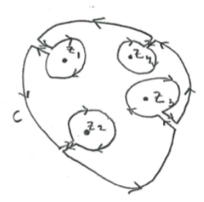
 = 2\pi i \sum_{j=1}^n \underset{z=z_j}{\rm Res} f(z)}") We have derived the Residue theorem, a very important result.
We have derived the Residue theorem, a very important result.
The residues can be obtained from
Expanding
as a Laurent series and taking the coefficient or, more easily,using a pocket formula for a pole of order
 (can be verified trivially)
  = \underset{z\rightarrow z_0}{\lim} \frac{1}{(n-1)!} \left(\frac{d}{dz}\right)^{n-1} [(z-z_0)^n f(z)]}")
In the quite often encountered special case of a simple pole  at we have
 =\frac{a_{-1}}{(z-z_0)} + a_0 +\cdots") and
and  = \underset{z\rightarrow z_0}{\lim} (z-z_0) f(z).") Let us now use these results for the evaluation of the Green's function.
Let us now use these results for the evaluation of the Green's function.
Evaluation of the Green's function
We can finally come back to our initial problem of calculating the Green's function. We would like to calculate =\int_{-\infty}^\infty dq \underbrace{\frac{q e^{iqr}}{(k+i\epsilon)^2-q^2}}_{f(q)}.")
Since ^2-q^2=(k+i\epsilon-q)(k+i\epsilon+q)") , the poles of
, the poles of ") are at
are at  and
and  , or
, or  and since
 =\frac{-q e^{iqr}}{(q-q_+)(q-q_-)} = -\frac{q e^{iqr}}{q_+-q_-} \left(\frac{1}{q-q_+} - \frac{1}{q-q_-}\right),") the poles at
the poles at  are simple poles of order 1. Let us calculate the residues:
  &=\underset{q\rightarrow q_\pm}{\lim} \frac{(-q) e^{iqr}}{(q-q_+)(q-q_-)}=\frac{-q_{\pm} e^{iq_\pm r}}{\underbrace{q_{\pm}-q_{\mp}}_{=2q_\pm}}\\
&=-\frac{1}{2} e^{iq_\pm r}.\end{aligned}") These are the residues of at .
These are the residues of at .
Wait! We have a simple integral over real values of . Where is the contour? The trick is to consider the integral over the real axis as part of a closed contour that closes along the complex plane as shown in the following picture (where we have chosen  ):
): 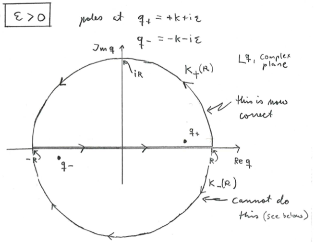
We should hence "close" the contour along the upper or lower complex half-plane. But which one should we use? This we see below. Either way, we can see that one of the poles is inside the contour , and the other one is outside. Anyway, the idea is the following: the residue theorem says  &= \ointctrclockwise_C dq f(q) \\&= \underset{R\rightarrow \infty}{\lim} \bigg[\int_{-R}^R dq f(q) + \underset{\text{\parbox{4cm}{$K_+(R)$ or $K_-(R)$\\semicircle at $|q|=R$}}}{\int dq f(q)}\mkern-54mu\bigg].\end{aligned}")
The first term inside the square brackets is the one we wish to compute. Now our aim is to choose the contour ") or
or ") so that the second integral vanishes. Let us choose first , i.e., close the contour in the upper half-plane:
so that the second integral vanishes. Let us choose first , i.e., close the contour in the upper half-plane: 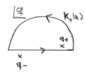
In this case, the pole  is inside , and
  is outside it. In other words,
  = 2\pi i \underset{q=q_+} {\rm Res} f(q) - \underset{R \rightarrow \infty}{\lim} \int_{K_+(R)} dq f(q).")
For ") , we can set
, we can set  ,
,  . Let us show that the contour integral along vanishes as
  . We have
 ) &= \frac{-R e^{i\varphi} e^{iRr\cos(\varphi)} e^{-Rr \sin(\varphi)}}{R^2 e^{i2\varphi}-(k+i\epsilon)^2}\\
&=\frac{-e^{i(-\varphi+Rr\cos\varphi)}}{R(1-(q_+/R)^2 e^{-i2\varphi})} e^{-Rr \sin(\varphi)}.\end{aligned}") Now take the limit . The absolute value of
Now take the limit . The absolute value of ") tends to
tends to |\xrightarrow{R\rightarrow \infty} \frac{1}{R} \exp[-\underbrace{Rr\sin \varphi}_{\text{\parbox{1.5cm}{$\ge 0$ since $\varphi \in [0,\pi]$}}}] \rightarrow 0.")
The integral along contour ") running along the upper half-plane therefore vanishes: note that the length of the contour is
running along the upper half-plane therefore vanishes: note that the length of the contour is  , and hence increases linearly with an increasing
  . However, the integrand vanishes exponentially with an increasing . Exponential function wins a linear one, and thus the result vanishes. We can see why we have to close the contour through the upper half plane, as for we would have
  (again ) and
  The integral along the lower half-plane would hence not vanish for .
In general which half-plane to close the contour depends on the case. For exponential functions with poles in the upper half-plane, we can prove the
Jordan's lemma: If | \le M(R)") , when
, when  ,
,  (upper half-plane), and
  \overset{R\rightarrow \infty}{\rightarrow} 0") , then
, then } g(z) e^{ikz}dz =0.")
Proof, using  and hence
  for a fixed :
 } g(z) e^{ikz} dz = \int_0^\varphi d\varphi i R e^{i\varphi} g(Re^{i\varphi}) e^{+ikR\cos \varphi} e^{-kR\sin \varphi}\\
&\Rightarrow |\int_{K_+(R)} g(z) e^{ikz}| \le \int_0^\pi d\varphi |iR e^{i\varphi} g(Re^{i\varphi}) \underbrace{e^{-ikR\cos \varphi}}_{\text{phase, }|.|=1} e^{-kR\sin(\varphi)}|\\
&=R\int_0^\varphi |g(Re^{i\varphi})| e^{-kR\sin(\varphi)}\\
&\overset{|g(z)| \le M(R)}{\le} R M(R) \int_0^\varphi d\varphi e^{-kR \sin \varphi} = 2 R M(R) \int_0^{\pi/2} d\varphi e^{-kR \sin \varphi}\\
&\overset{\sin \varphi \ge 2 \varphi/\pi}{\le} 2R M(R) \int_0^{\pi/2} d\varphi e^{-kR 2\varphi/\pi}\\
&=2RM(R) \frac{\pi}{2kR} (1-e^{-kR}) = \frac{\pi M(R)}{k} (1-e^{-kR}) \xrightarrow[M(R)\rightarrow 0]{R\rightarrow \infty} 0.\hfill _\square\end{aligned}")
Now let us apply Jordan's lemma to our problem: =\underbrace{\frac{-q}{q^2-(k+i\epsilon)^2}}_{g(q)} e^{iqr},") and we have that
and we have that |=R^{-1}|1-(q/R)^2e^{-i2\varphi}|^{-1} \le 1/R=M(R) \rightarrow 0") , so it fulfills the assumptions. This means that as , the integral of of the contour over the upper half-plane vanishes. Moreover, from the equation for the Green's function we have for
, so it fulfills the assumptions. This means that as , the integral of of the contour over the upper half-plane vanishes. Moreover, from the equation for the Green's function we have for =\int_{-\infty}^\infty dq f(q) = 2\pi i \underset{q=q_+}{\rm Res} f(q) = 2\pi i (-\frac{1}{2} e^{iq_+ r}) = -\pi i e^{i(k+i\epsilon)r}.")
In other words, the Green's function is =\frac{I_k^{\epsilon>0}}{4\pi^2 r i} = -\frac{1}{4\pi} \frac{e^{i(k+i\epsilon)r}}{r} \xrightarrow{\epsilon \rightarrow 0^+} -\frac{1}{4\pi} \frac{e^{ikr}}{r}}") Let us quickly check what would happen with the choise
Let us quickly check what would happen with the choise  . In this case the pole at
  would be outside and the pole inside it:
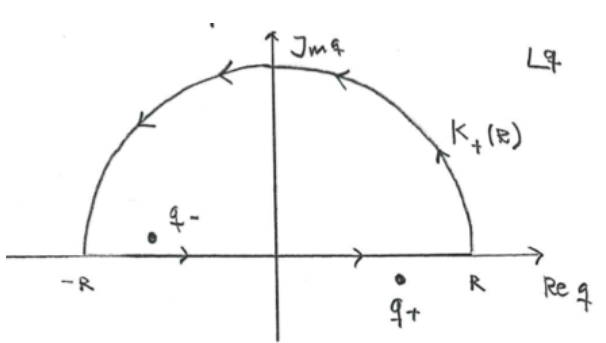
Now you should show that we get =-\pi i e^{-i(k+i\epsilon)r}") and the corresponding Green's function would be
and the corresponding Green's function would be =-\frac{1}{4\pi} \frac{e^{-ikr}}{r}") In other words,
In other words, =-\frac{1}{4\pi} \frac{e^{\pm ikr}}{r}.") Next, we show that it is
Next, we show that it is  that we want for the scattering problem, to describe an outgoing spherical wave.
Integral equation for potential scattering (IEPS)
Now, finally, substitute the above Green's function back to the integral equation for scattering, still allowing for either sign of . We get
=\phi_{\mathbf k}({\mathbf r})-\frac{1}{4\pi} \int d^{(3)} {\mathbf r}' \frac{e^{\pm ik|{\mathbf r}-{\mathbf r}'|}}{|{\mathbf r}-{\mathbf r}'|} U({\mathbf r}') \Psi_{\mathbf k}({\mathbf r}')}")
Here  \neq 0") in some vicinity of
in some vicinity of  . We should check the boundary condition at (not
  ) and choose the Green's function (+ or -) accordingly. Therefore, we should assume
  , and expand:
 ^2} = kr\sqrt{1-\frac{2{\mathbf r}\cdot {\mathbf r}'}{r^2}+\underbrace{\left(\frac{r'}{r}\right)^2}_{\rightarrow 0}}\\
&\approx kr\left(1-\frac{1}{2} 2 \underbrace{\frac{{\mathbf r}}{r}}_{\hat e_r} \cdot \frac{{\mathbf r}'}{r}+o\left(\left(\frac{r'}{r}\right)^2\right)\right)\\
&=kr-\underbrace{k\hat e_r}_{\equiv {\mathbf k}'} \cdot {\mathbf r}'.\end{aligned}") Note that we identified (defined) here the wave vector of the scattered particle,
Note that we identified (defined) here the wave vector of the scattered particle,  . As we are describing elastic scattering (energy of the incoming particle equals that of the outgoing particle), it has the same magnitude as the incoming particle, but a different direction.
Inserting this expansion into the integral equation for potential scattering yields in the lowest order  \overset{r\rightarrow \infty}{=}\phi_{\mathbf k}({\mathbf r})-\frac{e^{\pm ikr}}{r} \frac{1}{4\pi} \int d^3 {\mathbf r}' e^{\mp i{\mathbf k}' \cdot {\mathbf r}'} U({\mathbf r}') \Psi_{\mathbf k}({\mathbf r}').") Comparing this to the desired form, we find that in order to get the proper behavior, we have to choose in the Green's function
Comparing this to the desired form, we find that in order to get the proper behavior, we have to choose in the Green's function  .
.
Now recall that =\frac{1}{(2\pi)^{3/2}} e^{i{\mathbf k}\cdot {\mathbf r}}.") Moreover, comparing to the boundary condition, we can find an expression for the scattering amplitude
Moreover, comparing to the boundary condition, we can find an expression for the scattering amplitude =-\frac{(2\pi)^{3/2}}{4 \pi} \int d^{(3)} {\mathbf r}' \underbrace{e^{-i{\mathbf k}' \cdot {\mathbf r}'}}_{(2\pi)^{3/2} \phi_{{\mathbf k}'}^*({\mathbf r}')} U({\mathbf r}') \Psi_{\mathbf k}({\mathbf r}')") or
or =-2 \pi^2\int d^{(3)} {\mathbf r}' \phi_{{\mathbf k}'}^*({\mathbf r}') U({\mathbf r}') \Psi_{\mathbf k}({\mathbf r}')}") This we need for the calculation of the differential scattering cross section.
This we need for the calculation of the differential scattering cross section.
Solving the IEPS: Born approximation
Let us then solve the IEPS via an iteration method, using the fact that the integral equation contains ") on both sides of the equation. Let us hence substitute the left hand side to the right hand side. We get
on both sides of the equation. Let us hence substitute the left hand side to the right hand side. We get &=\phi_{\mathbf k}({\mathbf r})+\int d^{(3)}{\mathbf r}' G_{\mathbf k}({\mathbf r}-{\mathbf r}') U({\mathbf r}') \phi({\mathbf k}')\\
&+\int d^{(3)}{\mathbf r}' d^{(3)} {\mathbf r}'' G_{\mathbf k}({\mathbf r}-{\mathbf r}') U({\mathbf r}') G_{\mathbf k}({\mathbf r}'-{\mathbf r}'') U({\mathbf r}'') \Psi_{\mathbf k}({\mathbf r}'').\end{aligned}")
Substituting repeatedly to this equation hence generates the Born series of &=\phi_{\mathbf k}({\mathbf r})+\int d^{(3)}{\mathbf r}' G_{\mathbf k}({\mathbf r}-{\mathbf r}') U({\mathbf r}') \phi({\mathbf k}')\\
&+\int d^{(3)}{\mathbf r}' d^{(3)} {\mathbf r}'' G_{\mathbf k}({\mathbf r}-{\mathbf r}') U({\mathbf r}') G_{\mathbf k}({\mathbf r}'-{\mathbf r}'') U({\mathbf r}'') \phi_{\mathbf k}({\mathbf r}'') + \dots.\end{aligned}") Note that each new term contains a higher-order power of
Note that each new term contains a higher-order power of ") . It is hence an expansion in
. It is hence an expansion in  .
.
Let us write the scattering amplitude in a similar series. For illustration, let us define the wave vector of the incoming particle or "initial state wave vector" by  and that of the outgoing particle or "final state wave vector" by
  . The Born series of the scattering amplitude is
 =&-2\pi^2 \int d^{(3)}{\mathbf r}_1 \phi_{{\mathbf k}_f}^*({\mathbf r}_1) U({\mathbf r}_1) \Psi_{{\mathbf k}_i}({\mathbf r}_1)\\
=&-2\pi^2 \int d^{(3)} {\mathbf r}_1 \phi_{{\mathbf k}_f}^*({\mathbf r}_1) U({\mathbf r}_1) \phi_{{\mathbf k}_i}({\mathbf r}_1)\\
&-2\pi^2 \int d^{(3)} {\mathbf r}_1 d^{(3)} {\mathbf r}_2 \phi_{{\mathbf k}_f}^*({\mathbf r}_2) U({\mathbf r}_2) G_{\mathbf k}({\mathbf r}_2-{\mathbf r}_1) U({\mathbf r}_1) \phi_{{\mathbf k}_i}({\mathbf r}_1)\\
&-2\pi^2 \int d^{(3)} {\mathbf r}_1 d^{(3)} {\mathbf r}_2 d^{(3)} {\mathbf r}_3 \phi_{{\mathbf k}_f}^*({\mathbf r}_3) U({\mathbf r}_3) G_{\mathbf k}({\mathbf r}_3-{\mathbf r}_2) U({\mathbf r}_2) G_{\mathbf k}({\mathbf r}_2-{\mathbf r}_1) U({\mathbf r}_1) \phi_{{\mathbf k}_i}({\mathbf r}_1) + o(U^4).\end{aligned}") We can interpret this graphically and physically as follows:
We can interpret this graphically and physically as follows: 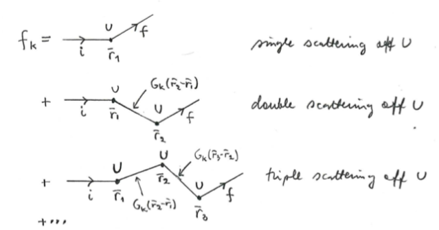
The Green's function ") is also called the propagator, which describes the propagation of a free particle from
is also called the propagator, which describes the propagation of a free particle from  to
to  . The interpretation of the Born series is thus that
  consists of a series of processes containing
  scattering events, where the incoming particle scatters off at
  , after which it moves as a free particle to the point
  , where it scatters off again, and so on. Obviously, if is very weak relative to the incident energy
 ") of the scattering particle(s), the contribution from multiple scatterings to the total scattering amplitude is small. In this case only the first term in the Born series is of relevance.
of the scattering particle(s), the contribution from multiple scatterings to the total scattering amplitude is small. In this case only the first term in the Born series is of relevance.
It can be shown that the Born series converges for all , if ") does not have bound states, i.e., is weak enough, and for (sufficiently) large , if
does not have bound states, i.e., is weak enough, and for (sufficiently) large , if  \xrightarrow{r\rightarrow \infty} 1/r^p") , where
, where  and
and  \xrightarrow{r \rightarrow 0} 1/r^s") , where
, where  . We can then define the
Born approximation = the first term in the Born series for ")
 = -2\pi^2 \int d^3 \mathbf r \phi^*_{\mathbf k_f}(\mathbf r)U(\mathbf r)\phi_{\mathbf k_i}(\mathbf r)=-\frac{1}{4\pi}\int d^3 {\mathbf r} e^{i(\mathbf k_i-\mathbf k_f)\cdot \mathbf r} U(\mathbf r).")
Let us examine this further by defining the momentum exchange vector }") By straightforward trigonometry (see the picture) one can show that
By straightforward trigonometry (see the picture) one can show that  Note that the momentum exchange vector depends on the angle . Using we can hence write the Born approximated form of the scattering amplitude in terms of the Fourier transform of the potential
  \equiv {\cal F}[U({\mathbf r})] = \frac{1}{(2\pi)^{3/2}} \int d^3 \mathbf r e^{-i{\mathbf q}\cdot {\mathbf r}} U({\mathbf r})") and hence
and hence  = -\frac{1}{4\pi} \int d^{(3)} {\mathbf r}e^{-i{\mathbf q}\cdot {\mathbf r}} U({\mathbf r}) = -\frac{(2\pi)^{3/2}}{4\pi}\tilde U({\mathbf q})}")
For a spherically symmetric potential, =V(r)") we have
we have &=-\frac{1}{4\pi} \frac{2\mu}{\hbar^2} \int \underbrace{d^{(3)} {\mathbf r}_1}_{d \cos \theta_1 d\varphi_1 r_1^2 dr_1} \exp(-i\underbrace{{\mathbf q}\cdot {\mathbf r}_1}_{qr_1\cos(\theta_1)})V(\mathbf{r}_1)\\
&=-\frac{1}{4\pi} \frac{2\mu}{\hbar^2} 4\pi \int_0^\infty dr_1 r_1^2 V(r_1) \frac{1}{qr_1} \sin(qr_1).\end{aligned}")
So, for a spherically symmetric potential we have  \overset{V({\mathbf r})=V(r)}=f_B(\theta) = -\frac{2\mu}{\hbar^2} \int_0^\infty dr r V(r) \frac{\sin(qr)}{q}}") Remember that the -dependence is in
Remember that the -dependence is in  .
.
Yukawa potential is =v_0 \frac{e^{-\kappa r}}{r}}") The potential thus has a range
The potential thus has a range  . It described a screened Coulomb potential, massive photons, or for example serves as a crude model for the nuclear binding force in an atomic nucleus. The benefit of it is that it leads to easy integrals using elementary functions. In the exercises you will show that for the Yukawa potential
 =-\frac{2\mu v_0}{\hbar^2} \frac{1}{q^2+\kappa^2} = -\frac{2\mu v_0}{\hbar^2} \frac{1}{4k^2 \sin^2 \frac{\theta}{2} + \kappa^2}.") The differential cross section for elastic scattering off a Yukawa potential becomes in the Born approximation
The differential cross section for elastic scattering off a Yukawa potential becomes in the Born approximation |^2 = \frac{4\mu^2 v_0^2}{\hbar^4} \frac{1}{(4k^2 \sin^2\frac{\theta}{2}+\kappa^2)^2}.") For curiosity, let us take the limit
For curiosity, let us take the limit  , and set
 ") as in the Coulomb potential, recalling that
as in the Coulomb potential, recalling that  . We thus get
  Notice, however, that if we take the limit , we are stepping outside the validity region of the above approach, since the range of
  is infinite. In particular, integrating the above differential cross section over the angles yields
  . However, the above result for the differential cross section is nevertheless correct.
Phew! There are a lot of technical details in the above sections. What should you take along? Well, at least
Definition of the scattering problem, total and differential cross section
Quantum scattering problem and the scattering amplitude
Green's function and integral equation
Solving the scattering Green's function: small imaginary term into wave number; residue theorem (complex integration)
Using residue theorem to evaluate certain types of integrals
Once we have the Green's function, for "weak enough" potentials we can solve the scattering problem via Born series
Note how the Born approximated version couples to the scattering amplitude.
Partial wave analysis
Another useful technique for calculating scattering amplitudes is the partial wave analysis, for the important special case of a rotation symmetric scattering potential. In this case, it is useful to project the angular dependence of the scattered wave amplitude (and thereby the differential cross section) into an orthonormal set of functions, the spherical harmonics.
Let us start by considering a spherically symmetric scattering potential ") , i.e., it only depends on the distance from the origin of the potential. The solutions of the Schrödinger equation for such a potential are of the form
, i.e., it only depends on the distance from the origin of the potential. The solutions of the Schrödinger equation for such a potential are of the form  = \sum_{l=0}^\infty \sum_{m=-l}^{l} a_{lm} R_l(r) Y_{lm}(\Omega),") where we include only the scattering solutions, and thus ignore the bound states.
where we include only the scattering solutions, and thus ignore the bound states.
The scattering amplitude can then be obtained from =-\frac{(2\pi)^{3/2}}{4\pi} \int \overbrace{d^3 \mathbf r'}^{dr'r'^2 d\cos \theta' d\varphi'} e^{-i\overbrace{\mathbf k \cdot \mathbf r'}^{kr'\cos \theta'}} U(r) \psi_{\mathbf k}(\mathbf r').") Substituting the above solution yields integrals over the angle of the form
Substituting the above solution yields integrals over the angle of the form }_{\sim e^{-im\varphi}} = 0, \quad \text{if } m\neq 0.")
In other words, it is enough to take into account the Ansatz with  :
:  = \sum_{l=0}^\infty a_l R_l(r) Y_{l0}(\theta).") The problem has a rotation symmetry with respect to the axis parallel with the direction of the incoming beam, and thus there is no dependence. Then also the scattering amplitude only depends on .
The problem has a rotation symmetry with respect to the axis parallel with the direction of the incoming beam, and thus there is no dependence. Then also the scattering amplitude only depends on .
The radial Schrödinger equation reads -\frac{l(l+1)}{r^2}\right]R_l(r)+V(r) R_l(r)=\epsilon R_l(r)") For simplicity, denote again
For simplicity, denote again =2\mu V(r)/\hbar^2") and . Then the radial equation goes to the form
and . Then the radial equation goes to the form  + 2r R'(r) + [(kr)^2-l(l+1)]R(r) -r^2 U(r) R(r)=0.
\end{aligned}")
To solve the scattering problem, from the solutions to this equation we pick up the ones fulfilling the boundary condition at . Outside the range of the potential ") , the solution to the radial equation can be specified in terms of spherical Bessel functions and
, the solution to the radial equation can be specified in terms of spherical Bessel functions and ") :
:  = R_l(k,r) \overset{r \rightarrow \infty}{=} A(l,k) j_l(kr) + B(l,k) n_l(kr).
\end{aligned}") For small argument, the two spherical Bessel functions have different behavior,
For small argument, the two spherical Bessel functions have different behavior, ") staying regular at the origin, whereas
staying regular at the origin, whereas ") diverges as
diverges as  . In the absence of the scattering potential (free particle), we should hence have
 \rightarrow 0") . For non-zero , however, we need to include also this part, but the size of the coefficient
. For non-zero , however, we need to include also this part, but the size of the coefficient ") measures the "strength" of scattering. In what follows, we quantify this strength with the scattering phase shift.
measures the "strength" of scattering. In what follows, we quantify this strength with the scattering phase shift.
For a large argument, the two spherical Bessel functions behave as  &\overset{kr \rightarrow \infty}{\rightarrow} \frac{1}{kr} \sin\left(kr-\frac{l\pi}{2}\right)\\
n_l(kr) &\overset{kr \rightarrow \infty}{\rightarrow} -\frac{1}{kr} \cos\left(kr-\frac{l\pi}{2}\right).
\end{aligned}")
They hence are phase shifted by  with respect to each other. Let us use this to define
  \overset{r\rightarrow \infty} = A(l,k) \left[j_l(kr) + \frac{B(l,k)}{A(l,k)} n_l(kr)\right] = A(l,k)\left[j_l(kr) - \tan(\delta_l(k)) n_l(kr)\right],
\end{aligned}") where
where ") is a phase shift determined by the scattering potential. For free particles, i.e., with
is a phase shift determined by the scattering potential. For free particles, i.e., with =0") ,
, =0") , and therefore
, and therefore  . For a non-zero scattering potential we then get a non-zero
  . This allows writing
  &\overset{r\rightarrow \infty}{=} \underbrace{\frac{A(l,k)}{\cos[\delta_l(k)]}}_{\equiv C(l,k)}
\frac{1}{kr}\left[\sin\left(kr-\frac{l\pi}{2}\right)\cos \delta_l(k)+\cos\left(kr-\frac{l\pi}{2}\right)\sin \delta_l(k)\right]\\
&=C(l,k) \frac{1}{kr} \sin\left[kr-l\frac{\pi}{2} +\delta_l(k)\right].
\end{aligned}")
The whole wave function is hence of the form  = \sum_l R_l(r) Y_{l0}(r) \overset{r\rightarrow \infty}{=} \sum_{l=0}^\infty a_l C(l,k) \frac{\sin\left[kr-\frac{l\pi}{2}+\delta_l(k)\right]}{kr} Y_{l0}(\theta).") The spherical harmonic functions are
The spherical harmonic functions are  = \sqrt{\frac{(2l+1)}{4\pi}} P_l(\cos \theta),") where
where ") are Legendre polynomials. In other words,
are Legendre polynomials. In other words,  \overset{r\rightarrow \infty}{=} \sum_{l=0}^\infty a(l,k) \frac{\sin[kr-l\pi/2+\delta_l(k)]}{kr} P_l(\cos \theta)
\end{aligned}") and
and =a_l C(l,k) \sqrt{(2l+1)/4\pi}") . Let us furthermore use
. Let us furthermore use =(e^{ix}-e^{-ix})/(2i)") to get
to get  \overset{r\rightarrow \infty}{=} \sum_{l=0}^\infty a(l,k) \frac{1}{kr} \frac{1}{2i} \left[e^{ikr} \underbrace{e^{-il\pi/2}}_{(-i)^l} e^{i\delta_l(k)}-e^{-ikr} \underbrace{e^{il\pi/2}}_{i^l} e^{-i\delta_l(k)}\right]P_l(\cos \theta)
\end{aligned}") or
or
 \overset{r\rightarrow \infty}{=} & \frac{e^{ikr}}{r} \sum_{l=0}^\infty \left[\frac{a(l,k)}{2ik} (-i)^l e^{i\delta_l} P_l(\cos \theta)\right]\\
-& \frac{e^{-ikr}}{r} \sum_{l=0}^\infty \left[\frac{a(l,k)}{2ik} i^l e^{-i\delta_l} P_l(\cos \theta)\right].
\end{aligned}") The asymptotic total wave function is hence a sum of outgoing and incoming spherical waves (first and second line).
The asymptotic total wave function is hence a sum of outgoing and incoming spherical waves (first and second line).
Comparing to the asymptotic wave describing scattering, we see that the incoming plane wave term  must contain a series of both outgoing and incoming spherical waves. This can be seen by the Legendre series of the plane wave (show this as an exercise):
 i^lj_l(kr) P_l(\cos \theta)
\end{aligned}")
Using the asymptotic form of at  again allows writing
  i^l \frac{1}{kr} \sin(kr-l\pi/2)P_l(\cos \theta)\\
&=\frac{e^{ikr}}{r} \sum_{l=0}^\infty (2l+1)\frac{P_l(\cos \theta)}{2ik}-\frac{e^{-ikr}}{r} \sum_{l=0}^\infty i^{2l} (2l+1)\frac{P_l(\cos \theta)}{2ik}.
\end{aligned}") This allows writing the asymptotic scattering wave function as as
This allows writing the asymptotic scattering wave function as as  \overset{r \rightarrow \infty}{=} &\frac{e^{ikr}}{r} \left[\frac{1}{(2\pi)^{3/2}} f_k(\theta) + \frac{1}{(2\pi)^{3/2}} \sum_{l=0}^{\infty} \frac{2l+1}{2ik} P_l(\cos \theta)\right]\\
-& \frac{e^{-ikr}}{r} \frac{1}{(2\pi)^{3/2}} \sum_{l=0}^\infty \frac{(2l+1)i^{2l}}{2ik} P_l(\cos \theta)
\end{aligned}") This we can now compare to the general asymptotic solution of the Schrödinger equation. This comparison allows identifying the different coefficients for incoming and outgoing scattering waves.
This we can now compare to the general asymptotic solution of the Schrödinger equation. This comparison allows identifying the different coefficients for incoming and outgoing scattering waves.
Let us use the fact that the Legendre polynomials form an orthogonal basis. Their coefficients in the two expressions must therefore match. From the coefficients of the incoming waves ( ) we get
 =\frac{(2l+1)i^l}{(2\pi)^{3/2}} e^{i\delta_l(k)}}.") On the other hand, the coefficients of the outgoing waves yield
On the other hand, the coefficients of the outgoing waves yield ^{3/2}} f_k(\theta) + \frac{1}{(2\pi)^{3/2}} \sum_l \frac{2l+1}{2ik} P_l(\cos \theta) = \sum_l \frac{a(l,k)}{2ik} (-i)^l e^{i\delta_l} P_l(\cos \theta).")
Substituting ") from the boxed formula above and simplifying yields the partial wave expansion of the scattering amplitude
from the boxed formula above and simplifying yields the partial wave expansion of the scattering amplitude  = \frac{1}{k} \sum_{l=0}^\infty (2l+1) f_l(k) P_l(\cos \theta)}
\end{aligned}") with the partial wave amplitude
with the partial wave amplitude  = e^{i\delta_l(k)} \sin \delta_l(k).
\end{aligned}")
The differential cross section is then |^2 =\frac{1}{k^2} \left\lvert\sum_{l=0}^\infty (2l+1)f_l(k) P_l(\cos \theta)\right\rvert^2") Using the orthonormality relation for the Legendre polynomials,
Using the orthonormality relation for the Legendre polynomials,  P_{l'}(\cos \theta) =\frac{2\delta_{ll'}}{2l+1},")
we can express the total cross section in terms of the partial wave amplitudes or scattering phase shifts  |f_l(k)|^2 = \frac{4\pi}{k^2} \sum_{l=0}^\infty (2l+1)\sin^2 \delta_l(k).}")
In other words, we have expressed the scattering amplitude ") and the cross section in terms of partial waves, each of which carries a specific amount of angular momentum
and the cross section in terms of partial waves, each of which carries a specific amount of angular momentum ") . The solutions of the radial Schrödinger equations are determined from the scattering potential , and thus it determines the scattering phase shifts and the partial wave amplitude
. The solutions of the radial Schrödinger equations are determined from the scattering potential , and thus it determines the scattering phase shifts and the partial wave amplitude =e^{i\delta_l(k)} \sin \delta_l(k)") .
.
Such a partial wave expansion is a useful method for computing and when there are only a few relevant terms in the sum over  . This is the case particularly when the energy (and thereby wave number ) of the incoming wave is small. Thinking classically: if the range of is
  , then
  if i.e.,
  . Then also
  and the
  term is the most important.
Quantum mechanically, the potential showing up in the radial Schrödinger equation is  Here shows the range of the potential. For small
 ") , the centrifugal barrier
, the centrifugal barrier }{r}") for
for  prevents the particle from entering the scattering region
  . Therefore, scattering takes place only for .
Remember the nomenclature for the scattering to the different partial waves:
- : "
 -wave" scattering
  : "
: " -wave" scattering
 : "
: " -wave" scattering and so on
In the behaviour of  see the following qualitative difference between low-energy and high-energy scattering:
Small energy:
-wave scattering only (). Thus  e^{i\delta_0(k)} \sin \delta_0(k) \underbrace{P_0(\cos \theta)}_{=1} \right\rvert^2 = \frac{sin^2 \delta_0(k)}{k^2}") has no -dependence and is hence spherically symmetric.
has no -dependence and is hence spherically symmetric.Larger energy: more partial waves (
 ) involved. These now involve
 ") with . But
with . But &=1, \text{ for $\theta=0$, i.e., forward scattering}\\
P_l(\cos \theta=-1)&=(-1)^l, \text{ for $\theta=\pi$, i.e., backward scattering}
\end{aligned}") In other words, forward scattering is amplified with increasing energy. This also makes intuitively sense, right?
In other words, forward scattering is amplified with increasing energy. This also makes intuitively sense, right? 
Optical theorem
Let us check the optical theorem from the partial wave expansion of the scattering amplitude. Taking its imaginary part and setting  yields
  &= \frac{1}{k} \sum_{l=0}^\infty (2l+1) {\rm Im}\left[\underbrace{e^{i\delta_l(k)}}_{\cos \delta_l+i\sin \delta_l} \sin \delta_l(k)\right]\underbrace{P_l(1)}_{=1}\\
&=\frac{1}{k} \sum_{l=0}^\infty (2l+1) \sin^2 \delta_l(k).
\end{aligned}")
Using the expression of the total cross section in terms of the partial waves we then get  = \frac{4\pi}{k} {\rm Im} f_k(\theta=0)}") similar to the result obtained above.
similar to the result obtained above.
Example: hard sphere scattering
Consider a hard-sphere potential of the form  = \begin{cases} \infty, \quad r \le a\\ 0, \quad r>0. \end{cases}") In the region
In the region  the solution of the radial Schrödinger equation is
 =A(l,k) j_l(kr) + B(l,k) n_l(kr)") whereas in the region
whereas in the region  it is
it is =0") .
.
Requiring continuity at  we then get
  j_l(ka)+B(l,k) n_l(ka)=0") or
or }{A(l,k)} = -\frac{j_l(ka)}{n_l(ka)} = -\tan \delta_l(k).")
The total cross section is hence  \underbrace{\sin^2 \delta_l(k)}_{\frac{\tan^2 \delta_l}{1+\tan^2 \delta_l}}\\
&=\frac{4\pi}{k^2} \sum_{l=0}^\infty (2l+1) \frac{j_l^2(ka)}{j_l^2(ka) + n_l^2(ka)}.
\end{aligned}")
This is the general solution for the cross section and hence applies for any spherical harmonic and radius of the sphere. However, let us gain a bit more understanding to the result by considering the low-energy limit (). We need there small-argument expansions of the spherical harmonics, yielding  &= 2^l x^l \sum_{s=0}^\infty \frac{(-1)^s (s+l)! x^{2s}}{s! (2s+2l+1)!} \overset{x\rightarrow 0}{\rightarrow} \frac{2^l l!}{(2l+1)!} x^l\\
n_l(x) &= \frac{(-1)^{l+1}}{2^l x^{l+1}} \sum_{s=0}^\infty \frac{(-1)^s (s-l)!}{s!(2s-2l)!} x^{2s} \overset{x\rightarrow 0}{\rightarrow} \frac{-(2l)!}{2^l l!}x^{-(l+1)}.
\end{aligned}") Using these results for the expression in the total cross section then yields
Using these results for the expression in the total cross section then yields }{j_l^2(ka)+n_l^2(ka)} \approx \frac{j_l^2(ka)}{n_l^2(ka)} \approx \left(\frac{2^l l! 2^l l!}{(2l+1)!(2l)!} x^{l+l+1}\right)^2 = \frac{1}{(2l+1)^2} \left(\frac{2^l l!}{(2l)!}\right)^4 x^{4l+2}.")
The total elastic cross section at low energies is hence !}\right)^4 \underbrace{(ka)^{4l+2}}_{\ll 1}.") The largest term is , which yields
The largest term is , which yields  In other words, the cross section is the total surface area of the sphere, not just the
  "seen" by the beam coming from the left. The latter would be the "billiard ball" hard sphere scattering cross section for classical particles. In other words, the quantum mechanical particle waves "feel" their way around the whole hard sphere, whereas classical particles only would see the head-on cross section:
These are the current permissions for this document; please modify if needed. You can always modify these permissions from the manage page.