# i.-introduction-to-qm-ii

I. Reminder of QM I

This course is about advanced quantum mechanics, trying to bridge the gap between the basic knowledge you obtained in the first course on quantum mechanics, and topics developed within the 20th century and whose understanding also help you grasp much of today's research literature. Before we dwell into the topics of the course, let us start with a reminder of what you should have learned in the previous course. I do not assume that you would know all of the following by heart. Rather, each topic should at least ring a bell, that you have heard it before, and after reading the sentences you should at least understand what they say. If not, you can go back to the introductory books and read those topics which seem hard.

Density matrices are an exception to this: they may not have been introduced in earlier courses. This is why this text includes a bit longer introduction to them.

The following consists of a brief reminder of topics in QM I (first six chapters of Griffiths' book).

# a.1-wave-function-and-probability

1.1 Wave function and probability

(See also postulates of quantum mechanics).

Crucial concepts:

Time dependent state vector (wave function) $\Psi(t) \in {\cal H}$ , where ${\cal H}$ is a Hilbert space (vector space with a well-defined inner product and where sequences converge to an element inside that space). In QM, state vectors are often denoted with the Dirac notation: $|\psi\rangle$ . The conjugate of $|\psi\rangle$ is $\langle \psi |$ . The inner product between two state vectors $\psi$ and $\phi$ is a complex number, and it is denoted as $\langle \psi | \phi \rangle = \langle \phi | \psi \rangle^*$ .

Observables described by Hermitian operators $\hat A$ acting on state vectors in ${\cal H}$ : $\hat A |\psi\rangle = |\phi\rangle$ . For example, position $\hat {\mathbf r}$ , momentum $\hat {\mathbf p}$ ( $\hat {\mathbf p} \cong \frac{\hbar}{i} \nabla_{\mathbf r}$ , $\hat {\mathbf r} \cong i\hbar \nabla_{\mathbf p}$ ), kinetic energy $\hat T=\frac{\hat{\mathbf p}^2}{2m}$ , total energy operator (Hamiltonian) $H=\hat T + V(\hat x)$ , angular momentum $\hat L=\hat {\mathbf r} \times \hat {\mathbf p}$ . The hat symbol $\hat .$ is often dropped unless one wants to make a distinction between operators and complex numbers.

Expectation value of observables in state $\psi$ : $\langle \hat A \rangle = \langle \psi | \hat A | \psi \rangle \in {\mathbb R}$ .

Representations of the state vector. The state vector can be represented in terms of the spectrum of a given $\hat A$ . Typically used representations are position representation $\psi(x) = \langle x | \psi \rangle$ , $\hat x |x\rangle = x |x\rangle$ and momentum representation $\psi(p)=\langle p | \psi\rangle$ , $\hat p |p\rangle=p|p\rangle$ . (Here and denote one of the coordinates, similar relations exist for each coordinate.)

Momentum and position are canonically conjugate variables, which means that the position and momentum representations are related via a Fourier transformation ( is the dimension of the vectors, the prefactor ensures normalization) $\begin{equation*}|{\mathbf p}\rangle = \frac{1}{(2\pi\hbar)^{d/2}} \int d^d \mathbf{r} e^{i {\mathbf p} \cdot {\mathbf r}/\hbar}|{\mathbf r}\rangle. \end{equation*}$ This implies the gradient representation for ${\mathbf{\hat p}}$ : $\begin{equation*} \mathbf{\hat p}|{\mathbf p}\rangle = {\mathbf{p}}|{\mathbf p}\rangle = \frac{1}{(2\pi\hbar)^{d/2}} \int d^d{\mathbf r} \mathbf{p} e^{i {\mathbf p} \cdot {\mathbf r}/\hbar}|{\mathbf r}\rangle = \frac{1}{(2\pi\hbar)^{d/2}} \int d^d \mathbf{r} (-i\hbar \mathbf{\nabla}) e^{i {\mathbf p} \cdot {\mathbf r}/\hbar}|{\mathbf r}\rangle = -i\hbar \mathbf{\nabla} |\mathbf p\rangle. \end{equation*}$

Schrödinger equation. The time dependence of the state vector is governed by the dynamical equation $i\hbar \partial_t |\Psi(t)\rangle = \hat H |\Psi(t)\rangle.$ We can write it also in position representation by multiplying from the left by $\langle {\mathbf r} |$ and denoting $\Psi({\mathbf r},t)=\langle {\mathbf r} | \Psi(t)\rangle$ $i \hbar \partial_t \Psi({\mathbf r},t) = \langle {\mathbf r} | \frac{\hat p^2}{2m} |\Psi(t)\rangle + V({\mathbf r}) \Psi({\mathbf r},t)= \left[-\frac{\hbar^2}{2m} \nabla_{\mathbf r}^2 +V({\mathbf r})\right]\Psi({\mathbf r},t).$

One consequence of the canonical commutation relations is the uncertainty principle: one cannot measure canonically conjugate variables simultaneously accurately, but the values of the two quantities have an intrinsic uncertainty: $\sqrt{\langle (\hat x-\langle \hat x\rangle)^2\rangle} \sqrt{\langle (\hat p-\langle \hat p\rangle)^2\rangle} \gtrsim \frac{\hbar}{2}$

This can be generalized to an arbitrary pair of operators $\hat A$ and $\hat B$ : $\sigma_A^2 \sigma_B^2 \gtrsim \left(\frac{1}{2i} \langle [\hat A,\hat B]\rangle\right)^2,$ where $\sigma_A^2 = \langle (\hat A-\langle \hat A\rangle)^2\rangle$ corresponds to the variance of the measurements of $\hat A$ over a given state and $[\hat A,\hat B]=\hat A \hat B-\hat B \hat A$ is the commutator between operators $\hat A$ and $\hat B$ .

# a.2-time-independent-schrödinger-equation

1.2 Time-independent Schrödinger equation

If the Hamiltonian is independent of time, we can solve the time-dependent Schrödinger equation with the Ansatz $|\Psi(t)\rangle = e^{-iE t/\hbar} |\psi\rangle$ , where $|\psi\rangle$ is independent of time and satisfies $H|\psi\rangle = E |\psi\rangle.$ The quantity is the (conserved) energy of the state $|\psi\rangle$ , it is an eigenvalue of the Hamiltonian , and $|\psi\rangle$ is the corresponding eigenvector.

The time-indepedent Schrödinger equation is often posed as a problem of finding the position representation of $|\psi\rangle$ . In other words, it amounts to finding a function $\psi({\mathbf r})$ that satisfies $-\frac{\hbar^2}{2m} \nabla_{\mathbf r}^2 \psi({\mathbf r}) + V(\mathbf{r}) \psi({\mathbf r})=E\psi({\mathbf r}).$

Infinite 1D square well (or a particle in a box) and discretized energies: for $x\in [0,a]$ , $\infty$ otherwise. Eigenenergies and (normalized) eigenstates of $\hat H$ are $\epsilon_n=\frac{\hbar^2 k_n^2}{2m} = \frac{n^2 \pi^2 \hbar^2}{2ma^2},\quad \psi_n(x)=\sqrt{\frac{2}{a}} \sin\left(\frac{n\pi}{a}x\right).$

Harmonic oscillator: potential energy $V(x)=\frac{1}{2}kx^2=\frac{1}{2} m\omega^2 x^2$ . Define the ladder operators or raising (+) and lowering (-) operators $\hat a_{\pm} = \frac{1}{\sqrt{2\hbar m \omega}} (\mp i \hat p + m \omega \hat x); \hat x = \sqrt{\frac{\hbar}{2m\omega}} (\hat a_++\hat a_-), \hat p = i\sqrt{\frac{\hbar m \omega}{2}} (\hat a_+-\hat a_-).$ The canonical commutation relations imply $[\hat a_-,\hat a_+]=1$ . The Hamiltonian can be written in terms of $H=\hbar \omega (\hat a_+ \hat a_-+1/2)$ . Energy eigenvalues are $\epsilon_n = (n+1/2)\hbar \omega$ , eigenstates $|n\rangle$ satisfy $a_+ |n\rangle = \sqrt{n+1} |n+1\rangle$ , $a_- |n\rangle = \sqrt{n} |n-1\rangle$ . The ground state is as $a_- |0\rangle = 0$ .

Free particle for which is described by plane wave states. They are also position representations of states with a well-defined momentum, because if , $\hat H$ commutes with $\hat p$ , and thus $\hat p$ is a conserved quantity, see also Subsection on symmetry below. $\langle x | \psi\rangle = A e^{ikx} + B e^{-ikx}.$ Here $k=\sqrt{2mE}/\hbar>0$ is the wave number. Generally plane waves are not normalizable unless we include proper boundary conditions (to be discussed more in the context of time-dependent theory). Sometimes we can also use the concept of a wave packet that contains a (typically Lorentzian) weight function with several values of . Note that a state with a given corresponds to a momentum $p=\hbar k$ . The first term describes a wave "going" to the right and the second term a wave "going" to the left.

Tunneling through a $\delta$ -function or a square potential. Divide the Ansatz function to parts: $\psi=\psi_L(x) \theta(x_L-x) + \psi_W(x) \theta(x-x_L) \theta(x_R-x) + \psi_R(x) \theta(x-x_R),$ where $\theta(x)$ is the Heaviside step function. 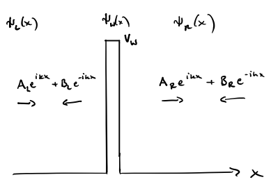In each part, the ansatz consists of left- and right-going states, i.e., $\psi_{L/W/R}=A_{L/W/R} e^{ik_{L/W/R}x} + B_{L/W/R} e^{-ik_{L/W/R}x},$ where $k_\alpha=\sqrt{2m(E-V_\alpha)}/\hbar$ . The coefficients $A_\alpha$ and $B_\alpha$ can be determined by matching wave functions and their derivatives at the boundaries (for the square well), or matching the difference of derivatives to the height of the $\delta$ -function. Finding the coefficients amounts to solving a scattering problem: a particle with amplitude coming from the left reflects with probability amplitude and transmits through with probability amplitude . Note that transmission is allowed even if the potential in the center exceeds the energy of the particle (). In that case transmission is called tunneling.

# a.3-formal-properties-of-state-vectors

1.3 Formal properties of state vectors

Identify state vectors with -component vectors $|\psi\rangle \cong \vec{\psi}=\begin{pmatrix} \psi_1 & \psi_2 & \dots & \psi_n \end{pmatrix}^T \in {\mathbb C}^n,$ where can be (even incountably) infinite.

The vector representation is possible via specifying the state vector in terms of the eigenstates $|a_n\rangle$ of some (Hermitian) operator $\hat A$ , i.e., $\hat A = a_n |a_n\rangle$ . In this case we can also write (sum becomes an integral in the case of an incountable set) $|\psi\rangle = \sum_{j=1}^n \psi_j |a_j\rangle.$ The eigenvectors of Hermitian operators are orthogonal and can be chosen to be normalized, i.e., $\langle a_i | a_j \rangle = \delta_{ij}$ . They hence form an orthonormal basis. This means that the above representation is unique and that the coefficients can be found from $\psi_j = \langle a_j | \psi \rangle.$ (As for example in position/momentum representation.)

The above properties define the Hilbert space in which the state vector lives.

Basis functions can be used to generate a projection operator $\hat P_\alpha = |\alpha\rangle \langle \alpha |,$ where $|\alpha\rangle$ is assumed to be normalized. $\hat P_\alpha$ projects a given state to state $|\alpha\rangle$ , i.e., $\hat P_\alpha|\beta\rangle= |\alpha\rangle \langle \alpha | \beta \rangle= \langle \alpha | \beta \rangle |\alpha\rangle$ . It also satisfies $\hat P^2=\hat P$ , i.e., double projection is equal to a single projection.

Resolution of unity. Representation of a unit operator $\sum_\alpha \hat P_\alpha = \hat 1,$ where the sum goes over states spanning an orthonormal basis for a given Hilbert space (prove it!).

# a.4-quantum-mechanics-in-three-dimensions

1.4 Quantum mechanics in three dimensions

In spaces of dimension higher than one, the position representation of the Schrödinger equation becomes a partial differential equation with several coordinates. This typically calls for proper Ansatz functions that respect the symmetry of the problem (typically the symmetry of the potential or of the boundary conditions).

Special case: spherically symmetric potential, i.e., a central potential. Write the Laplacian $\nabla^2$ in spherical coordinates ( $(x,y,z) \mapsto (r,\theta,\phi)$ ) $\nabla^2 = \frac{1}{r^2} \partial_r (r^2 \partial_r)+\frac{1}{r^2 \sin(\theta)} \partial_\theta (\sin(\theta) \partial_\theta) + \frac{1}{r^2 \sin^2 \theta} (\partial_\phi^2).$ For the central potential $V({\mathbf r})=V(r)$ , an appropriate Ansatz is $\psi(r,\theta,\phi)=R(r) Y(\theta,\phi)$ . Plugging it to the Schrödinger equation gives

$\begin{aligned} \frac{1}{R} \partial_r (r^2 \partial_r R)-\frac{2mr^2}{\hbar^2}[V(r)-E]&=l (l+1)\\ \frac{1}{Y} \left\{\frac{1}{\sin(\theta)} \partial_\theta (\sin(\theta) \partial_\theta Y)+\frac{1}{\sin^2 \theta} \partial_\phi^2 Y\right\}&=-l(l+1),\end{aligned}$ where l(l+1) is a constant. The term on the rhs of the first equation describes an effective centrifugal potential $\hbar^2/(2m) l(l+1)/r^2$ .

Solution for the angular part described by two integer-valued quantum numbers, (azimuthal quantum number) and (magnetic quantum number), $m=-l,-l+1,\dots l$ : spherical harmonics (no need to remember the exact form) $|lm\rangle = Y_l^m(\theta,\phi)=A_{lm} e^{im\phi} P_l^m(\cos \theta),$ where $A_{lm}$ is a constant, and is the associated Legendre function.

Solution depends on . If the centrifugal potential dominates it, one can typically try spherical bessel functions as an Ansatz.

Hydrogen atom is an example of a system with a central potential $V(r)=-e^2/(4\pi \epsilon_0 r)$ . In the -equation, one gets a new quantum number, $n=1,2,3,\dots$ (principal quantum number). The eigenenergies are $E_n=-\left[\frac{m}{2\hbar^2} \left(\frac{e^2}{4\pi \epsilon_0}\right)^2\right] \frac{1}{n} \equiv \frac{E_1}{n^2},$ where eV.

Angular momentum operator $\hat {\mathbf L}=\hat {\mathbf r} \times \hat {\mathbf p}$ , , , . The components do not commute (identify $1 \cong x$ , $2 \cong y$ , $3 \cong z$ ): $[L_i,L_j]=i\hbar \epsilon_{ijk} L_k,$ where $\epsilon_{ijk}$ is the completely antisymmetric tensor or Levi-Civita symbol satisfying $\epsilon_{123}=\epsilon_{231}=\epsilon_{312}=1$ , $\epsilon_{132}=\epsilon_{321}=\epsilon_{213}=-1$ , and 0 otherwise. The angular momentum operators have well-defined eigenvalues: $\hat {\mathbf L}^2 |lm\rangle = \hbar^2 l (l+1)|lm\rangle$ , and $\hat L_z |lm\rangle = \hbar m |lm\rangle$ , where $l,m \in {\mathbb Z}$ , $m=-l, \dots l$ . Note that $|lm\rangle$ are the spherical harmonics.

Spin encodes an internal degree of freedom of particles, analog to the particle revolving around itself. Spin operators behave somewhat analogously to angular momentum operators, but they permit half-integer eigenvalues: $\hat S^2 |sm_s\rangle=\hbar^2 s(s+1) |sm_s\rangle$ , $S_z |sm_s\rangle = \hbar m_s | sm_s\rangle$ , $s=0, 1/2, 1, 3/2, \dots$ , $m_s=-s, -s+1, \dots s$ .

Spin 1/2 is an often studied special case. It is encoded by two eigenstates $|+1/2\rangle$ and $|-1/2\rangle.$ Spin operators are often represented by Pauli matrices, $S_j=\hbar \sigma_j/2$ , $\sigma_x=\begin{pmatrix} 0 & 1\\1 & 0\end{pmatrix} \quad \sigma_y=\begin{pmatrix} 0 & -i\\i & 0\end{pmatrix} \quad \sigma_z=\begin{pmatrix} 1 & 0\\0 & -1\end{pmatrix}.$ (Learn by heart). Pauli matrices satisfy $[\sigma_i,\sigma_j]=2i\epsilon_{ijk} \sigma_k$ .

Presence of spin can be demonstrated in the Stern-Gerlach experiment, where applying an inhomogeneous magnetic field separates particles with different

# a.5-identical-particles

1.5 Identical particles

(We will return to this in QM II B)

Bosons (particles with integer spin) and fermions (half integer spins), spin statistics theorem
Fermions: Pauli exclusion principle
Atoms: shell filling, Hund's rules (not really used in this course)
Solids: start from free electron gas, define Fermi energy (highest allowed energy), band structure from Bloch's theorem (not used here, but in the materials physics courses)
Quantum statistics: chemical potential, temperature, Fermi-Dirac and Bose-Einstein distributions (discussed more in the statistical physics course)

# a.6-time-independent-perturbation-theory

1.6 Time-independent perturbation theory

(We will discuss time-dependent perturbation theory later in QM II A)

System with a Hamiltonian $H=H^0+\lambda H'$ , where the spectrum of H^0 is somehow known, and is a (time independent) perturbation. Idea is to develop a perturbation series, both on eigenfunctions and -energies of : $\begin{aligned} |\psi_n\rangle&=|\psi_n^0\rangle+\lambda |\psi_n^1\rangle + \lambda^2 |\psi_n^2\rangle + \cdots\\ E_n&=E_n^0 + \lambda E_n^1 + \lambda^2 E_n^2\end{aligned}$ Here $H^0 |\psi_n^0\rangle = E_n^0 |\psi_n^0\rangle$ .

First-order theory (non-degenerate spectrum ): $\begin{aligned} |\psi_n^1\rangle &= \sum_{m\neq n} \frac{\langle \psi_m^0 | H' |\psi_n^0\rangle}{E_n^0-E_m^0} |\psi_m^0\rangle\\ E_n^1&=\langle \psi_n^0 | H' | \psi_n^0\rangle.\end{aligned}$ The term $\langle \psi_m^0 | H' |\psi_n^0\rangle$ is called the matrix element of in the basis defined by $\{|\psi_n\rangle\}_n$ .

Second-order energies $E_n^2=\sum_{m\neq n} \frac{|\langle \psi_m^0 | H' |\psi_n^0\rangle|^2}{E_n^0-E_m^0}.$
Degenerate spectrum: find the basis spanning the degenerate states, write all matrix elements of within this basis, and diagonalize. Often leads to lifting of degeneracies.
Hydrogen atom: lifting of degeneracies due to magnetic field due to spin-orbit coupling (more in QMII B), Zeeman effect (more later in this course) and hyperfine splitting due to coupling of proton and electron spins.

# subs:symmetry

1.7 Addition: symmetry in QM

System described by a Hamiltonian has a given (discrete or continuous) symmetry if the symmetry operator $\hat K$ commutes with : [H,K]=0 . This commutation is equivalent with

The value for the observable related to $\hat K$ is time independent, i.e., constant of motion.
and share the same eigenstates (but naturally not usually the same eigenvalues)

# a.8-postulates-of-quantum-mechanics

1.8 Postulates of quantum mechanics

With the knowledge above, let us state the theory of quantum mechanics in terms of postulates, i.e., things that really cannot be derived, but which we more or less use as starting points.

Information as precise as possible of the physical system at a given time is contained in the state vector $|\psi(t)\rangle$ . The state vectors are elements of a linear vector space which possesses an inner product.

Corresponding to each observable, i.e., a physical measurable quantity , there is a linear and hermitian operator $\hat A$ , which operates on the state vectors $|\psi\rangle$ of the state vector space. [In this case $\hat A$ has an eigenvalue equation $\hat A |a\rangle = a |a\rangle$ , real eigenvalues , and orthogonal (orthonormal) eigenvectors $|a\rangle$ which form a basis.]

In the measurement of an observable , only the eigenvalues of the operator $\hat A$ are possible measurement results.

If the system is in a state $|\psi\rangle$ and an observable is measured, the probability to obtain a value is $|c_a|^2=|\langle a | \psi\rangle|^2$ , i.e., the expectation value of an observable is $\langle A\rangle=\langle \psi | \hat A |\psi\rangle$ .

Canonical quantization. The operators $\hat x_j$ and $\hat p_k$ , which correspond to the classical quantities for location and momentum, fulfill the canonical commutation rules $[\hat x_j,\hat x_k]=[\hat p_j,\hat p_k]=0; \quad [\hat x_j,\hat p_k]=i\hbar \delta_{jk}\quad \text{$\hbar=\frac{h}{2\pi}$; $j,k=1,2,3$}.$

The time evolution of the system state obeys the Schrödinger equation $i\hbar \frac{d}{dt} |\psi(t)\rangle = \hat H |\psi(t)\rangle.$ The Hamilton operator $\hat H$ is formed from the classical Hamilton function $H(t,{\mathbf p},{\mathbf x}) \mapsto \hat H(t,\hat{\mathbf p},\hat{\mathbf x})$ via canonical quantization.

1.9 Density matrix

This may be a new topic to many of you

Above we describe the quantum phenomena using the state vector or wave function description. This is adequate when dealing with closed, isolated systems. Often, however, we have access only to part of the relevant system, or we have a limited knowledge of the state of the system. For example, let us assume that the system is with probability p_i in state $|\psi_i\rangle$ ( $i=1,2,\dots$ ). In this case it is described with a density operator $\rho=\sum_i p_i |\psi_i\rangle \langle \psi_i|,$ where $|\psi_i\rangle$ and $\{p_i\}$ are normalized: $\langle \psi_i|\psi_i\rangle=1$ , $\sum_i p_i=1$ . If there are only a finite number of states involved, $\rho$ can be represented with a matrix, and therefore the term density matrix is also often used.

With this definition, the expectation value of observables can be expressed straigthforwardly, $\begin{aligned} \langle O \rangle &\equiv \sum_i p_i \underbrace{\langle \psi_i|\hat O}_{\text{insert $\hat 1=\sum_k |\psi_k\rangle \langle \psi_k|$}} |\psi_i\rangle \\ &=\sum_{i,k} p_i \langle \psi_i|\psi_k\rangle \langle \psi_k | \hat O | \psi_i\rangle \\ &=\sum_k \langle \psi_k | \hat O \underbrace{\sum_i |\psi_i \rangle p_i \langle \psi_i|}_{\rho}|\psi_k\rangle\\ &=\sum_k \langle \psi_k|\hat O \rho|\psi_k\rangle \equiv {\rm Tr}[\hat O \rho].\end{aligned}$ Expectation value can hence be calculated from a trace over the operator product of $\hat O$ and the density operator $\rho$ : $\boxed{\langle O \rangle = {\rm Tr}[\hat O \rho]}$ In addition, the density operator has three important properties:

It is Hermitian: $\rho^\dagger = \rho$
It has a unit trace: ${\rm Tr}[\rho]=1$ .
$\rho$ is a positive operator: for any state $|\phi\rangle$ , $\langle \phi |\rho |\phi\rangle \ge 0$ .

Property (i) is easy to prove from the definition of $\rho$ : $\rho^\dagger = \sum_i p_i^* |\psi_i\rangle \langle \psi_i| = \sum_i p_i |\psi_i\rangle \langle \psi_i| = \rho,$ because $p_i \in {\mathbb R}$ is a probability and not a probability amplitude.

Property (ii) comes from the normalization: $\begin{aligned} {\rm Tr}[\rho] &\equiv \sum_k \langle \psi_k | \rho |\psi_k\rangle = \sum_{k,i} p_i \langle \psi_k | \psi_i\rangle \langle \psi_i | \psi_k\rangle\\ &=\sum_{i} p_i \langle \psi_i| \underbrace{\sum_k|\psi_k\rangle \langle \psi_k |}_{=\hat 1} |\psi_i\rangle = \sum_i p_i \underbrace{\langle \psi_i | \psi_i\rangle}_{=1} = \sum_i p_i = 1.\end{aligned}$

Moreover, the positivity condition is proven as $\begin{aligned} \langle \phi | \rho | \phi\rangle &= \sum_i p_i \langle \phi|\psi_i\rangle \underbrace{\langle \psi_i | \phi\rangle}_{=\langle \phi|\psi\rangle^*}\\ &=\sum_i \underbrace{p_i}_{\ge 0} \underbrace{|\langle \phi| \psi_i\rangle|^2}_{\ge 0} \ge 0.\end{aligned}$ This also means that all eigenvalues of $\rho$ are bound to be larger than or equal to zero (they are real because $\rho$ is Hermitian).

# iii.8.1-pure-and-mixed-states

1.9b Pure and mixed states

Let us consider the density matrix corresponding to the superposition state $|\psi\rangle = a |0\rangle + b |1\rangle,$ where $|0\rangle$ and $|1\rangle$ are some normalized eigenstates. The density matrix is $\begin{aligned} \rho&=|\psi\rangle \langle \psi|=|a|^2 |0\rangle \langle 0| + |b|^2 |1\rangle \langle 1| + ab^* |0\rangle \langle 1| + ba^* |1\rangle \langle 0|\\ &\cong \begin{pmatrix} |a|^2 & ab^* \\ a^* b & |b|^2 \end{pmatrix} = \begin{pmatrix} \rho_{00} & \rho_{01} \\ \rho_{10} & \rho_{11} \end{pmatrix}.\end{aligned}$ In the second line we express the states with the two-component vector, $\psi=\begin{pmatrix} a \\ b\end{pmatrix}, \text{ i.e., } |0\rangle \cong \begin{pmatrix} 1 \\ 0\end{pmatrix}, |1\rangle \cong \begin{pmatrix} 0 \\ 1\end{pmatrix}.$ This density matrix should be contrasted to that of a mixed state that cannot be represented in terms of a single state vector. For example $\rho=\begin{pmatrix} \rho_{00} & 0\\0& \rho_{11}\end{pmatrix},$ where $\rho_{00}, \rho_{11}$ both are non-zero.

Pure states, which can be represented in terms of a single state vector, satisfy

A state described by $\rho$ is pure if and only if $\rho^2=\rho$ .

First, let us show that $\rho^2=\rho$ implies a pure state.

Let $\rho=\sum_i \lambda_i |\lambda_i\rangle \langle \lambda_i|$ be the spectral decomposition of $\rho$ . If $\rho^2=\rho$ , we have $\rho^2=\sum_i \lambda_i^2 |\lambda_i\rangle \langle \lambda_i| = \sum_i \lambda_i |\lambda_i\rangle \langle \lambda_i|.$ Because $|\lambda_i\rangle$ are orthonormal, this means $\lambda_i^2=\lambda_i$ for any . Therefore, $\lambda_i=1$ or $\lambda_i=0$ . But because ${\rm Tr}[\rho]=\sum_i \lambda_i=1$ , $\lambda_p=1$ for some , and $\lambda_{i\neq p}=0$ . Therefore $\rho=|\lambda_p\rangle \langle \lambda_p|$ is a pure state described by the state vector $|\lambda_p\rangle$ .

We can in fact simplify this requirement to consider only the trace:

$\rho$ is pure iff ${\rm Tr}[\rho^2]=1$ .

You can prove this as an exercise.

Entropy

John von Neumann showed that besides purity, the pure and mixed states can be distinguished by their entropy, defined as $S=-k_B {\rm Tr}[\rho \ln \rho].$ The trace of an operator is independent of the basis in which it is calculated. Therefore, the above can also be written as (check) $S=-k_B \sum_i p_i \ln p_i,$ where p_i is the probability of the density matrix being in state $|\psi_i\rangle$ .

It is straightforward to show that the entropy of a pure state vanishes, whereas it is non-vanishing (and ) for a mixed state.

The following sections are strictly speaking outside the course contents, but if you are interested to understand how density matrices are actually used in describing open quantum systems, you may study also them.

1.9c System and a bath, thermal density matrix

Here we consider an example where a quantum system (QS) is in contact with a bath, an environment to the QS containing a macroscopic number of degrees of freedom.

Let us consider a brief detour via classical thermodynamics. In equilibrium the bath is at temperature $T=1/(k_B \beta)$ , where k_B is the Boltzmann constant. In this case the probability for the state with energy E_i is $p_i=e^{-\beta E_i}/{\cal Z}$ , where the normalization constant ${\cal Z}$ is determined below. This means that $\rho=\sum_i p_i |\psi_i\rangle \langle \psi_i|,$ where $|\psi_i\rangle$ are eigenstates of the QS Hamiltonian, $H|\psi_i\rangle = E_i|\psi_i\rangle$ Hence $\rho=\frac{1}{\cal Z} \underbrace{\sum_i e^{-\beta E_i} |\psi_i\rangle \langle \psi_i|}_{\text{spectral representation of $e^{-\beta H}$}} \equiv \frac{e^{-\beta H}}{\cal Z}.$ Hence, such a thermal state is pure only at T=0 .

The mixed states illustrate a lack of information about the state of the full system. For example, in the thermal equilibrium state we have "lost" the information of the occupation of the bath microstates.

1.9d Reduced density operator

Let us consider a system composed of two parts, A and B. In the case the states of the two systems are pure and independent of one another, we can write the full state vector as $|\psi_{AB}\rangle = |\psi_A\rangle |\psi_B\rangle.$ In the vector language this means an outer product between $|\psi_A\rangle$ and $|\psi_B\rangle$ , often written also as $|\psi_A\rangle \otimes |\psi_B\rangle.$ In the vector representation, an outer product between, say, $2\times 1$ vectors is of the form $\begin{pmatrix} a\\b\end{pmatrix} \otimes \begin{pmatrix} c\\d\end{pmatrix} = \begin{pmatrix} ac\\ad\\bc\\bd\end{pmatrix}.$ If the basis states for A,B are $|0\rangle_{A,B}$ and $|1\rangle_{A,B}$ , the basis states of the outer product are $|n\rangle_A |m\rangle_B \cong |nm\rangle, \quad (n,m \in \{0,1\}).$ The density matrix for an outer product state is $\rho_{AB}=\rho_A \otimes \rho_B = |\psi_A\rangle |\psi_B\rangle \langle \psi_B| \langle \psi_A|.$ Let us introduce the concept of a partial trace. Assume that we can access only the state of the system A. In this case we should sum over, or trace out the states in system B. We define

The reduced density operator of system A is $\rho^A = {\rm Tr}_B \rho_{AB} \equiv \sum_i \langle \psi_i^B | \rho_{AB} | \psi_i^B\rangle,$ where $\{|\psi_i^B\rangle\}$ forms a complete orthonormal set of states in B.

Note that $\rho^A$ still satisfies the density operator properties (i)-(iii) on page (show this as an exercise). For a product state $\rho_{AB}=\rho_A \otimes \rho_B$ , we get $\rho^A={\rm Tr}_B \rho_A \otimes \rho_B = \rho_A \underbrace{{\rm Tr}_B \rho_B}_{=1} = \rho_A.$ However, not all states can be represented as product states. For example, let us consider the Bell state $|\psi\rangle_{\rm Bell}=(|00\rangle + |11\rangle)/\sqrt{2}$ . Its density matrix is $\rho_{\rm Bell}=|\psi\rangle_{\rm Bell} \langle \psi|_{\rm Bell}=\frac{1}{2}(|00\rangle \langle 00| + |11\rangle \langle 11| + |00\rangle \langle 11| + |11\rangle \langle 00|).$ Now let us consider its partial trace $\begin{aligned} {\rm Tr}_B \rho_{\rm Bell}&=\langle 0|_B \rho_{\rm Bell} |0\rangle_B + \langle 1|_B \rho_{\rm Bell}|1\rangle_B\\ &=\frac{1}{2}(|0\rangle_A\langle 0|_A+|1\rangle_A \langle 1|_A) \cong \frac{1}{2}\begin{pmatrix}1 & 0\\0&1\end{pmatrix} = \rho^A.\end{aligned}$ Although the full $\rho_{\rm Bell}$ represents a pure state, $\rho^A$ is a mixed state. Check this: ${\rm Tr}[\rho^2]={\rm Tr}\left[\frac{1}{4}\begin{pmatrix}1&0\\0&1\end{pmatrix}\right]=\frac{1}{2} \neq 1.$ The fact that a reduced density matrix of a pure state becomes a mixed state is a signature of quantum entanglement.

1.9e Liouville-von Neumann equation and quantum master equation

Let us consider the time dependence of the density matrix in the Schrödinger picture. There we have $i\hbar \frac{d}{dt} |\psi(t)\rangle = H|\psi(t)\rangle, {\text{ and }} -i\hbar \frac{d}{dt} \langle \psi(t)| = \langle \psi(t)|H.$ Therefore, $\begin{aligned} i\hbar \frac{d\rho}{dt} \overset{(*)}{=}& i\hbar \sum_i p_i [|\dot \psi_i\rangle \langle \psi_i|+|\psi_i\rangle \langle \dot \psi_i|]\\ =&\sum_i p_i(H|\psi_i\rangle \langle \psi_i|-|\psi_i\rangle \langle \psi_i| H)=H\rho -\rho H \equiv [H,\rho].\end{aligned}$ Note that the first equality (*) applies only in a closed system, where the p_i are time independent. A reduced density operator may have time dependent p_i . This case is discussed more below. Nevertheless, for a closed system we obtained the Liouville-von Neumann equation $\boxed{\frac{d\rho}{dt}=-\frac{i}{\hbar}[H,\rho]}.$ Note that this has a very similar form as the Heisenberg equation of motion for an operator $\hat A_H(t)$ , $\frac{d\hat A_H(t)}{dt} = \frac{i}{\hbar}[H,\hat A_H],$ except that the prefactor of the commutator has an opposite sign.

The formal solution of the Liouville-von Neumann equation can be expressed in terms of Schrödinger picture propagators $\begin{equation} \rho(t)=U_S(t,t_0) \rho(t_0) U_S^\dagger(t,t_0), \end{equation}$ where $U_S(t,t_0)=\exp\left(-\frac{i}{\hbar} \int_{t_0}^t H(t') dt'\right) \overset{H(t)={\rm const.}}{=}e^{-\frac{i}{\hbar} H(t-t_0)}.$ This can be directly proven by taking the derivative of both sides of Eq. (1) with respect to time and using the Liouville-von Neumann equation.

For a reduced density operator the interaction with the external system gives rise to an additional term describing the dynamics, i.e., for example in the above example system composed of subsystems A and B, $\frac{d\rho^A}{dt} = -\frac{i}{\hbar} [H_A,\rho^A]+{\cal L}[\rho^A(t)].$ The superoperator ${\cal L}[\rho^A(t)]$ is in general a nonlocal (in time) functional of $\rho^A(t)$ . This is the case in systems possessing memory. For example, you may consider the case where the interaction between A and B induces a transition between two states in A and simultaneously another transition in B (say, B is excited and A is de-excited). This event may trigger the inverse process at a later time. To maintain the correlation between these processes, ${\cal L}$ would have to be non-local.

However, in many cases it is sufficient to consider a Markovian environment, which does not have memory. In this case one can construct an approximate model for ${\cal L}$ . A typical choice is the Lindblad superoperator ${\cal L}$ of the form ${\cal L}=\sum_{k=1}^M \gamma_k \left(\hat L_k \rho \hat L_k^\dagger - \frac{1}{2}\{\hat L_k^\dagger \hat L_k,\rho\}\right),$ where is limited from above in the case of finite systems ( M<N^2-1 in the case of a system with basis states), $\gamma_k \ge 0$ is a rate for process , and $\hat L_k$ are called Lindblad operators. They are quite generally linear operators acting between states in subsystem .

Note that when ${\cal L}=0$ (usual Liouville-von Neumann equation), the time evolution is unitary ( $U_S^\dagger(t,t_0)U_S(t,t_0)=1$ ) and hence reversible. A non-zero ${\cal L}$ can describe an irreversible process. In this case the irreversibility arises from throwing out the knowledge of the microscopic degrees of freedom of the bath.

Examples of the use of the Lindblad superoperator are given for example on this wikipedia page.

One can show that the Lindblad superoperator maintains the three properties (i)-(iii) on page for $\rho$ :

follows from the fact that $({\cal L} \rho)^\dagger = {\cal L}\rho$ .
requires that $\frac{d{\rm Tr}\rho}{dt}={\rm Tr}\left[-\frac{i}{\hbar}[H,\rho]\right]+{\rm Tr}[{\cal L}\rho] \overset{?}{=}0.$ To see this, we need to show the "cyclic property of the trace": ${\rm Tr}[ABC]={\rm Tr}[BCA]={\rm Tr}[CAB],$ valid for arbitrary operators .

$\begin{aligned} {\rm Tr}[ABC]&\equiv \sum_i \langle \psi_i|ABC|\psi_i\rangle \\ &=\sum_{ijk}\langle \psi_i |A|\psi_j\rangle \langle \psi_j | B |\psi_k\rangle \langle \psi_k |C|\psi_i\rangle\\ &=\sum_{ijk}\langle \psi_j |B|\psi_k\rangle \langle \psi_k | C |\psi_i\rangle \langle \psi_i |A|\psi_j\rangle \equiv {\rm Tr}[BCA]\\ &=\sum_{ijk}\langle \psi_k |C|\psi_i\rangle \langle \psi_i | A |\psi_j\rangle \langle \psi_j |B|\psi_k\rangle \equiv {\rm Tr}[CAB].\end{aligned}$

Note that in general ${\rm Tr}[ABC]\neq {\rm Tr}[ACB]$ (why?).

Now proceeding with the proof of (ii), we find ${\rm Tr}[-\frac{i}{\hbar}[H,\rho]]=-\frac{i}{\hbar}{\rm Tr}[H\rho-\rho H]=0.$ Furthermore, $\begin{aligned} {\rm Tr}[{\cal L}\rho]&=\sum_k \gamma_k {\rm Tr}[\hat L_k \rho \hat L_k^\dagger-\frac{1}{2}\{\hat L_k^\dagger \hat L_k,\rho\}]\\ &=\sum_k \gamma_k {\rm Tr}[\hat L_k^\dagger \hat L_k \rho-\frac{1}{2}(\hat L_k^\dagger \hat L_k \rho + \rho \hat L_k^\dagger \hat L_k)]=0,\end{aligned}$ where we used the cyclic property of the trace.

Therefore, the Lindblad operator does not change the trace of $\rho$ .
Proving property (iii) is beyond the scope of this course. It was first proven by G. Lindblad in Commun. Math. Phys. 48, 119 (1976).

It can be shown that all Markovian (i.e., time-local) operators maintaining the properties (i)-(iii) are of the form $\dot \rho = -\frac{i}{\hbar}[H,\rho]+{\cal L}[\rho_A],$ where ${\cal L}$ is the one given above. This equation is called the quantum master equation. Note, however, that the presence of the environment can still affect the form of , i.e., the effective Hamiltonian of the system may get renormalized due to the environment.